

On this page
Solubility product questions feel abstract on paper: a tiny number, a square root, an answer in mol/L. In a simulation you can watch it happen. You tip salt into water, see it dissolve, and notice the moment when crystals start sitting at the bottom and the dissolved ion count stops rising. That moment is saturation, and Ksp tells you exactly when it arrives.
What does a salt solubility simulation show?
PhET at the University of Colorado makes a free simulation called Salts & Solubility. Its own description reads: "Add different salts to water, then watch them dissolve and achieve a dynamic equilibrium with solid precipitate" (PhET simulation listing). The learning goals PhET lists include ranking the solubility of different salts and calculating "the molarity of saturated solutions, and Ksp values".
The key thing to watch is the word "dynamic". At saturation, ions keep leaving the crystal and rejoining it. The rates match, so the counts stay level while particles keep moving. A static textbook diagram cannot show that. We built the Fermi Simulation Lab for ideas like this one that are easier to see than to read.
When does a solution become saturated?
Start with the definition. The equilibrium constant between a slightly soluble ionic solid and its ions in solution is called the solubility product, Ksp (OpenStax Chemistry 2e via LibreTexts). The same source gives the test: a solid begins to precipitate when the reaction quotient Q exceeds Ksp.
So while you are adding salt, compare Q (the product of the ion concentrations you have right now) with Ksp:
Q below Ksp: unsaturated, everything you add dissolves.
Q equal to Ksp: saturated, solid and ions in balance.
Q above Ksp: solid comes out until Q falls back to Ksp.
The solid itself does not appear in the expression, which is why Ksp for AgCl is simply [Ag⁺][Cl⁻]. Our post on why solids and pure liquids drop out of K explains the reason.
How does Ksp set the ion concentrations?
The numbers below use the 25°C values in the LibreTexts solubility constants table, which is taken from the CRC Handbook of Chemistry and Physics.
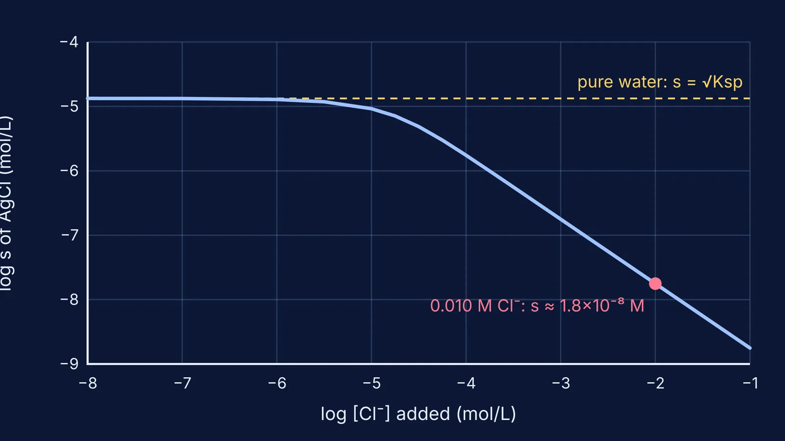
Silver chloride, AgCl (1:1). Ksp = 1.77 × 10⁻¹⁰. If s mol/L dissolves, [Ag⁺] = [Cl⁻] = s, so s² = 1.77 × 10⁻¹⁰ and s = 1.33 × 10⁻⁵ mol/L.
Lead iodide, PbI₂ (1:2). Ksp = 9.8 × 10⁻⁹. Now [Pb²⁺] = s and [I⁻] = 2s, so Ksp = s(2s)² = 4s³. That gives s = 1.35 × 10⁻³ mol/L, with [I⁻] = 2.70 × 10⁻³ mol/L. Forgetting to square the 2s is a common slip.
The trap: silver chromate, Ag₂CrO₄ (2:1). Ksp = 1.12 × 10⁻¹², smaller than AgCl's. Yet 4s³ = 1.12 × 10⁻¹² gives s = 6.5 × 10⁻⁵ mol/L, about five times more soluble than AgCl.
What does adding a common ion do?
The common ion effect is the drop in solubility when you add a substance that shares an ion with the dissolved salt (OpenStax Chemistry 2e via LibreTexts). Le Chatelier's principle predicts the direction. Ksp gives you the size.
Dissolve AgCl in 0.010 M NaCl instead of pure water. The chloride already there dominates, so [Cl⁻] ≈ 0.010 and s ≈ 1.77 × 10⁻¹⁰ ÷ 0.010 = 1.8 × 10⁻⁸ mol/L. Compared with 1.33 × 10⁻⁵ mol/L in pure water, that is roughly 750 times less AgCl in solution, using the same Ksp table.
The approximation holds because 1.8 × 10⁻⁸ is tiny next to 0.010. Always check that before you drop the s.
For PbI₂ in 0.10 M KI, [I⁻] ≈ 0.10, so s ≈ 9.8 × 10⁻⁹ ÷ 0.010 = 9.8 × 10⁻⁷ mol/L. Here the squared term matters again: you divide by 0.10², not 0.10.
How to use the simulation: five predictions to test
Write each prediction down before you run it.
Before adding any salt, predict which of two salts will saturate first, using s rather than Ksp.
Add salt slowly. Note the point where a solid first stays at the bottom. That is Q reaching Ksp.
Add twice as much salt beyond that point. Predict the dissolved ion counts. (They should not change.)
Add more water. Predict whether some solid dissolves. (It should, until the solution is saturated again.)
Do the common ion step on paper with the numbers above, then compare with what the simulation's equilibrium suggests.
If your hand calculation and the screen disagree, find the step where they split. For the full set of rules, including precipitation checks after mixing two solutions, read our solubility product guide on Ksp, the common ion effect and precipitation. And if you want to know when an animation helps more than a diagram, see what studies found about simulations and static diagrams.
When a numerical still will not come out, the Fermi Problem Library has worked problems with a step-by-step solver that explains the reasoning rather than printing an answer.


