

On this page
If you open a vapour pressure simulation, drop sugar into a beaker of water and watch the pressure gauge dip, you have seen Raoult's law at work. The more useful habit is to predict the reading before you press play, so the simulation checks your reasoning. Here is the equation, a prediction table, a worked example and a plan.
What does Raoult's law say about adding a solute?
Raoult's law: the partial pressure of any component of an ideal solution equals the vapour pressure of the pure component multiplied by its mole fraction in the solution, as stated in OpenStax Chemistry 2e.
A non-volatile solute such as sugar barely evaporates, so only the solvent counts: P = x(solvent) × P°. Since x(solvent) = 1 − x(solute), a little algebra gives the form you will see in exams: (P° − P) / P° = x(solute). In words, the fractional drop in vapour pressure equals the mole fraction of solute.
OpenStax gives the picture behind it: the solute decreases the surface area available to solvent molecules, which slows evaporation. Vapour pressure lowering is one of the four colligative properties, which depend on how many solute particles there are, not on what they are. Our guide to colligative properties and the van 't Hoff factor goes further, with worked freezing point problems and common slips.
How do you predict vapour pressure from mole fraction?
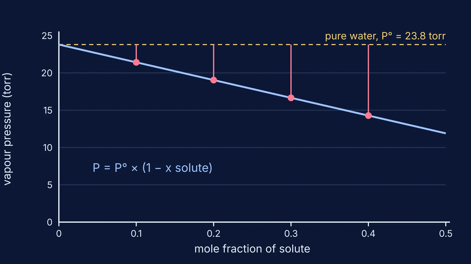
Pure water at 25 °C has a vapour pressure of 23.8 torr, according to the water properties table in OpenStax Chemistry 2e. Multiply that by the mole fraction of water, and write each prediction down before you run the simulation:
x(solute) = 0: P = 23.8 torr (pure water)
x(solute) = 0.10: P = 0.90 × 23.8 = 21.4 torr
x(solute) = 0.20: P = 0.80 × 23.8 = 19.0 torr
x(solute) = 0.40: P = 0.60 × 23.8 = 14.3 torr
Plot these and you get a straight line falling from P°. If the simulation's points bend away from it, the solution is not behaving ideally. Our post on ideal and non-ideal solutions explains why real mixtures drift.
Worked example, with one mole of glucose in a kilogram of water:
Moles of water: 1000 g ÷ 18.02 g/mol = 55.5 mol.
Moles of glucose: 180 g ÷ 180 g/mol = 1.00 mol.
x(solute) = 1.00 ÷ 56.5 = 0.0177.
P = (1 − 0.0177) × 23.8 = 23.4 torr. The drop is only about 0.4 torr, so set your simulation's scale to see it.
Why does boiling point rise when vapour pressure falls?
A liquid boils when its vapour pressure equals the pressure above it. The OpenStax table shows water reaching 760 torr at 100 °C (OpenStax water properties). The solution's vapour pressure curve lies below pure water's at every temperature, so it has to be heated past 100 °C to reach 760 torr. OpenStax states this directly: because the solute lowers vapour pressure, the solution's boiling point is higher.
For dilute solutions the rise is ΔTb = Kb × m, where m is molality. For water, Kb = 0.512 °C kg/mol (OpenStax Chemistry 2e). The glucose solution above is 1 mol/kg, so it boils about 0.51 °C higher, near 100.5 °C at 1 atm.
Why does freezing point drop?
On a phase diagram, the solution's solid-liquid line sits to the left of pure water's, OpenStax explains, and that leftward shift is the freezing point depression (OpenStax Chemistry 2e). One way to picture it: the ice that forms is pure water, so its vapour pressure does not change. The solution's vapour pressure has dropped, though, so the two only match at a lower temperature.
The formula is ΔTf = Kf × m, and for water Kf = 1.86 °C kg/mol, from the same OpenStax table of constants. The 1 mol/kg glucose solution freezes near −1.86 °C, a shift over three times the boiling point rise.
How should you run the simulation?
Use predict, observe, explain. Our look at what research says about interactive simulations covers why giving a simulation a prediction to test helps.
Note P° for the solvent at your chosen temperature.
Pick three solute amounts and convert each to a mole fraction on paper.
Write your predicted P for each one, then run the simulation.
Plot predicted against observed. A gap usually means you used grams instead of moles, or forgot to count ions.
Switch to a heating view and check that the solution reaches the outside pressure at a higher temperature.
Explain the result in one sentence, out loud.
The Fermi Simulation Lab has interactive simulations for ideas that are easier to see than to read, so you can practise the same predict-first habit there. If mole fraction or molality still feels shaky, the Fermi Concept Library has a lesson for each concept and shows where it fits on the map.


