

On this page
Functions wrapped in absolute values appear frequently in JEE Main and advanced mathematics, often creating sharp corners where a smooth curve once was. But putting the whole function inside the modulus lines behaves completely differently from putting just the x inside.
When you compare the graph of y = |f(x)| to y = f(|x|), you are watching the difference between changing the final output and altering the initial input. Knowing how to predict these changes without plotting every point will save you critical minutes in an exam. Here is how to predict what will happen to a standard quadratic equation.
How to graph y = |f(x)|?
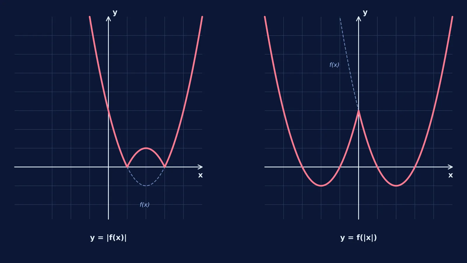
When the absolute value wraps the entire expression, it strictly affects the final y-value. The rule is simple: any part of the original graph that sits below the x-axis (where y is negative) is reflected across the x-axis so that it becomes positive. The parts already on or above the x-axis stay exactly where they are.
Take the quadratic function f(x) = x² − 4x + 3. This is a standard parabola that opens upwards, with roots at x = 1 and x = 3. Its lowest point is the vertex located at (2, −1).
If we want to graph y = |x² − 4x + 3|, the segment of the curve from x = 1 to x = 3 (which dips down to a y-value of −1) flips upwards. The vertex at (2, −1) reflects to become a sharp peak at (2, 1). The resulting graph looks like a rounded "W" resting on the x-axis.
This transformation radically changes the range of the function. While the original parabola reached down to −1, the range of y = |f(x)| is restricted to [0, ∞).
How to graph y = f(|x|)?
When the absolute value wraps only the x, it alters the input before the function can calculate anything. Because |x| is always positive or zero, the function never receives a negative number to process. It treats every negative x exactly as if it were the positive version of that number.
To sketch the graph of y = f(|x|):
Keep the part of the original graph where x ≥ 0 (the right side of the y-axis).
Delete the part where x < 0 (the entire left side).
Take the kept right side and reflect it across the y-axis to replace the deleted left side.
Applying this rule to f(|x|) = |x|² − 4|x| + 3, we start by keeping the right side of our original parabola. This right half includes the vertex (2, −1) and the roots at 1 and 3. Next, we mirror that exact shape onto the empty left side of the y-axis. The newly created left side will have roots at −1 and −3, with a second vertex at (−2, −1).
Because the left side is a perfect mirror of the right side, the final graph of y = f(|x|) is always symmetric across the y-axis. In mathematical terms, this transformation forces the result to become an even function.
If you struggle to visualise these overlapping transformations, you can build them step by step in the Simulation Lab. Seeing the original smooth curve overlaid directly with its modulus versions makes it much easier to spot where the reflections actually happen.
How do these transformations change the number of roots?
Exam problems rarely ask you to just draw the curve. Instead, they often ask you to count the number of solutions to an equation, which corresponds directly to the number of roots on the graph.
For y = |x² − 4x + 3|, the number of roots does not change. The curve still touches the x-axis at 1 and 3. The reflection only happens below the axis, leaving the crossing points alone.
By contrast, for y = |x|² − 4|x| + 3, mirroring the right half across the y-axis created two entirely new roots at −1 and −3. This gives the transformed equation four distinct roots in total.
Understanding this distinction is also critical for calculus problems involving differentiation. The sharp corners created by these modulus reflections are points where the graph is continuous but not differentiable. For |f(x)|, the non-differentiable points appear at the roots. For f(|x|), a non-differentiable corner often appears right on the y-axis.
If you are ever unsure When is ax² + bx + c positive for all x?, sketching out the reflections can immediately reveal whether a transformed quadratic will ever dip below the x-axis. And when you get stuck trying to set up the initial curve for a tough problem, Fermi's AI tutor can work out what you already know and teach through it, drawing the figure with you on a board.


