

On this page
If you connect a load — like a light bulb or a motor — to a real battery, the battery's own internal resistance fights you. If you make the load resistance too small, the battery wastes most of its power heating itself up. If you make it too large, the current drops and barely any power flows at all. The sweet spot in the middle is governed by a fundamental rule of circuit design.
What is the Maximum Power Transfer Theorem?
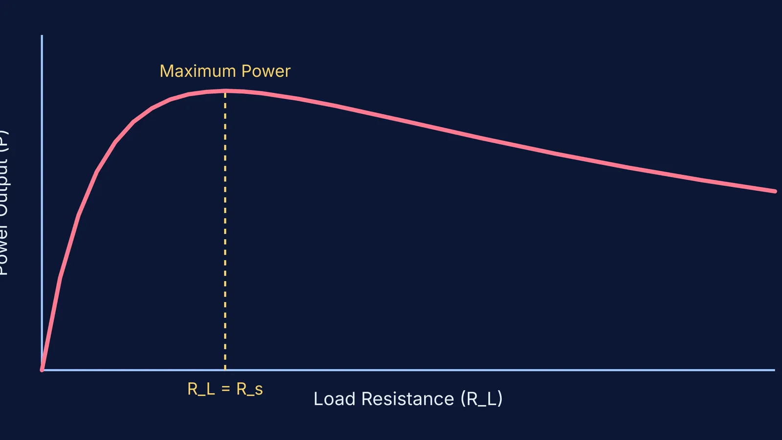
The Maximum Power Transfer Theorem defines how to extract the highest possible power from a source that has internal resistance. Published by Moritz von Jacobi in 1840 (Wikipedia), the theorem proves that peak power output occurs when the load resistance exactly equals the internal resistance of the source.
Because the load and the internal resistance are equal at this point, they share the voltage equally. This means that exactly 50% (Wikipedia) of the total power generated is wasted as heat inside the battery itself. You get maximum power, but you do not get maximum efficiency.
How to predict the maximum power transfer load resistance?
You can prove Jacobi's law yourself using standard calculus and Ohm's law. By expressing the power dissipated by the load as a function of its resistance, you can find the peak of the curve.
Here is a step-by-step worked example:
Write the current (I). For a voltage source (V) with internal resistance (r) and a load resistance (R), the current is I = V / (r + R).
Write the power equation. The power (P) transferred to the load is P = I²R.
Substitute the current. This gives P = V²R / (r + R)².
Take the derivative. To find the maximum, differentiate P with respect to R using the quotient rule: dP/dR = V² [ (r + R)² - 2R(r + R) ] / (r + R)⁴.
Set the derivative to zero. For dP/dR to be zero, the numerator must be zero: (r + R)² - 2R(r + R) = 0.
Solve for R. Dividing by (r + R) leaves r + R - 2R = 0, which simplifies to R = r.
This mathematical approach is the same one you use when tackling the Resistance of a tapered conductor: set up the physical relationship, apply calculus to find the limit or peak, and simplify the result.
Where do we use maximum power transfer in real life?
While the theorem is a staple of physics exams, it also drives the design of everyday technology. However, because of the strict 50% (Wikipedia) efficiency limit, engineers only use it when power is scarce and efficiency does not matter as much as extracting a usable signal.
For example, when connecting a microphone to an audio amplifier, the goal is to transfer the maximum possible signal power from the microphone (the source) to the amplifier (the load). Audio engineers use impedance matching to ensure the amplifier's input resistance matches the microphone's internal resistance. Wasting half the power is an acceptable trade-off to ensure the delicate audio signal is strong enough to process.
Conversely, you would never use maximum power transfer for a city's electrical grid. If a power plant tried to match its load to its internal resistance, it would lose half of its generated energy as heat, destroying its own generators in the process. For heavy power transmission, engineers keep the source resistance as close to zero as possible to maximize efficiency, not absolute power transfer.
How does a maximum power transfer load resistance simulation work?
Deriving the equation is one thing, but seeing the curve peak in real time builds a stronger intuition. If you are preparing for exams, visualizing how variables interact is often faster than re-deriving them under time pressure.
In the Fermi Simulation Lab, you can run an interactive simulation to test this theorem. You set the battery's internal resistance to a fixed value, then sweep the load resistance from near zero up to a large multiple of the internal resistance.
As you adjust the slider, the simulation plots a live power graph. You will see the curve rise sharply, hit a clear, rounded peak exactly where the load matches the internal resistance, and then slowly taper off as the resistance continues to grow.
This active testing bridges the gap between abstract algebra and physical circuits. When you know what the curve looks like, you can double-check your answers when solving complex networks using the Node potential method.


