

On this page
Matrix multiplication can often feel like a blind shuffle of rows and columns. You multiply a vector by a matrix, and a new vector pops out, as if by magic. But matrices are not just arbitrary grids of numbers; they are precise instructions for stretching, squashing and shearing the fabric of space. When you learn how to read those mathematical instructions visually, the concept of an inverse matrix transforms from a tedious calculation into a logical, predictable and highly satisfying geometric step.
What does a stretch and shear matrix do?
To see how this works, we can look at a two-dimensional space defined by a standard grid, using a simple unit square that sits squarely between 0 and 1 on the x and y axes. When you apply a matrix transformation to this space, you move the basis vectors (the foundational building blocks of the axes) to completely new positions, taking the square and every other shape on the plane with them.
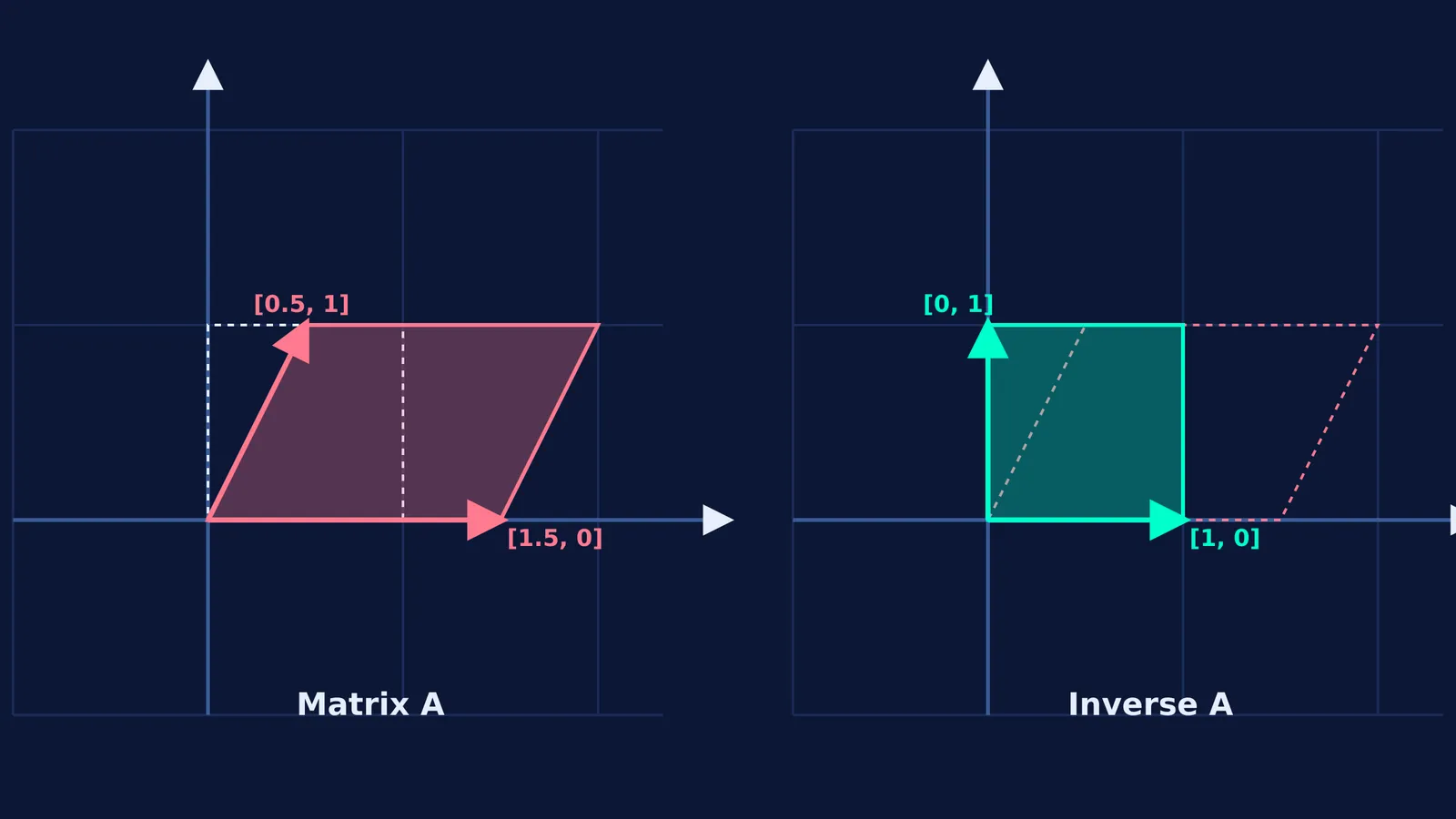
Let us test a transformation matrix, A, with the top row [1.5, 0.5] and the bottom row [0, 1]. We can break down its effect by looking at the individual columns.
The first column, [1.5, 0], tells us exactly where the x-axis unit vector lands. It stretches out along the horizontal axis by a factor of 1.5, making the space wider. The second column, [0.5, 1], tells us where the y-axis unit vector lands. It shifts slightly to the right by 0.5 units but crucially stays at the same vertical height, which is a horizontal shear.
When we apply this matrix to the entire plane, the original unit square becomes a wider, right-leaning parallelogram. The right side stretches outwards, and the top edge pushes smoothly to the right, completely warping the original geometry.
How does an inverse matrix undo a transformation visually?
Instead of jumping straight to the standard determinant formula to find the inverse, look at the transformed, leaning parallelogram and predict what physical steps must happen to restore the original, upright square.
Fix the stretch: The entire x-axis was stretched by a factor of 3/2. To bring it back to a standard length of 1, we must actively compress it by multiplying the horizontal distances by 2/3.
Fix the shear: The y-axis was pushed out to the right, causing the shape to lean. To straighten the geometry up, we must pull the top edge back to the left by exactly the same proportion.
Now, let us calculate the actual inverse matrix, A⁻¹, using standard algebra to see if our visual predictions hold true. First, the determinant is (1.5 × 1) − (0.5 × 0) = 1.5. To form the inverse, we swap the top-left and bottom-right numbers, flip the signs of the remaining two numbers, and finally divide everything by the determinant of 1.5.
The resulting inverse matrix has a top row of [2/3, −1/3] and a bottom row of [0, 1].
Read this new matrix visually just as we did before. The first column, [2/3, 0], compresses the x-axis exactly as we predicted. The second column, [−1/3, 1], pulls the top of the shape backwards to the left, perfectly reversing the earlier shear.
When you apply A⁻¹ to the stretched, leaning parallelogram, the visual result is immediate and elegant: the shape compresses horizontally, leans back to the left, and snaps perfectly back into the original unit square.
Why is visualising matrix transformations important?
Being able to independently predict these geometric moves changes how you check your work in a high-pressure exam scenario. If your calculated algebraic inverse has a positive number where it should clearly be pulling the shape to the left, you know you have made a sign error before you even finish solving the problem. Visual tools lock in this deep conceptual understanding; a 2025 study in *Pedagogical Constellations* showed that 80% of students who learned visually could formally justify their algebraic steps, whereas only 25% of traditional learners could do the same.
In the Fermi Simulation Lab, you can drag the basis vectors on an interactive plane to physically apply any combination of stretches, reflections, and shears. You can then ask Fermi's AI tutor to compute the corresponding inverse matrix and watch the simulation dynamically unwind your changes step by step. Seeing the geometry visually snap back builds an enduring intuition that raw algebra alone rarely provides.
Once you deeply understand what the inverse does geometrically, you can dive into adjoint and inverse of a matrix, or explore finding Aⁿ for a matrix by spotting the pattern to see exactly what happens when a single transformation repeats infinitely.


