

On this page
When you first meet integration by parts, it looks like a symbol-juggling trick. The formula ∫ u dv = uv − ∫ v du is printed in textbooks as an algebraic rule derived from the product rule of differentiation.
Because it is taught algebraically, students often treat it passively. You assign u and dv, substitute them in, and hope the new integral is easier than the old one. If you make a mistake, you have to start again.
But what if you could just see the formula as a shape?
How is integration by parts visualised as area?
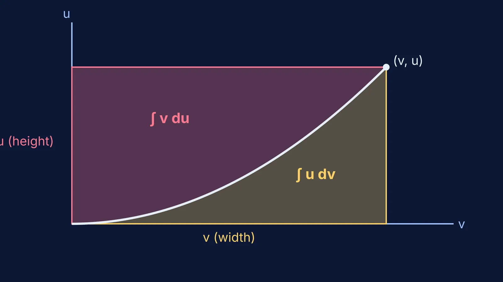
Instead of looking at the standard x-y plane, imagine a graph where the horizontal axis is v and the vertical axis is u. Any relationship between u and v can be plotted as a curve on this plane.
Pick a starting point on the curve, like the origin (0, 0), and an end point (v, u). If you draw a box from the origin to this point, you form a large rectangle.
The width of the rectangle is v.
The height of the rectangle is u.
Therefore, the total area of the rectangle is u × v.
This rectangle is sliced into two pieces by the curve you plotted:
The area below the curve: You can find this by adding up thin vertical strips. Each strip has a height of u and a tiny width of dv. This gives the integral ∫ u dv.
The area to the left of the curve: You can find this by adding up thin horizontal strips (similar to finding area using horizontal strips). Each strip has a width of v and a tiny height of du. This gives the integral ∫ v du.
How do you prove integration by parts geometrically?
Because these two areas perfectly assemble the total rectangle, their sum must exactly equal the total area.
Mathematically, you can state this relationship as: ∫ u dv + ∫ v du = uv
Rearrange the equation by moving one integral to the other side, and you have the classic formula: ∫ u dv = uv − ∫ v du
How does this help with inverse functions?
Visualising this geometry is particularly powerful when you are asked to integrate an inverse function, such as the natural logarithm, ln(x).
If you set u = ln(x) and dv = dx, then v = x. The integral you want to solve is ∫ ln(x) dx, which matches the ∫ u dv side of the geometric equation (the area below the curve).
Instead of guessing the algebraic steps, look at the rectangle. The total area is uv, which is x ln(x). The area to the left of the curve is ∫ v du. Since u = ln(x), we know that x = eᵘ, which means v = eᵘ. Integrating v with respect to u is suddenly very easy: the integral of eᵘ is just eᵘ, which equals x.
By simply subtracting the easy area (x) from the total rectangle area (x ln(x)), you get the answer: x ln(x) − x. The geometric method completely bypasses the standard algebraic integration steps.
Why does active learning work better for calculus?
Calculus can easily feel like a wall of abstract symbols, especially when you run into cyclic problems like integrating eᵃˣ sin bx where the formula loops back on itself. When you visualise integration by parts as an area, you move from passively following rules to actively manipulating ideas.
Educational research consistently shows the value of this shift. In a landmark study of undergraduate STEM courses published in the Proceedings of the National Academy of Sciences, researchers found that active learning leads to increases in examination performance that raise average grades by half a letter. Furthermore, students in traditional lecture setups were 55% more likely to fail compared to those engaged in active learning environments.
You can experience this active approach in the Fermi Simulation Lab. Here, interactive simulations for the ideas that are easier to see than to read allow you to predict how two areas add up to uv. You can drag the curve in real time and watch the integration by parts formula shift dynamically as a rectangle, solidifying the concept far better than a static textbook diagram.
How can you practice this active method?
If you want to test this geometric method yourself, follow this checklist the next time you face a difficult integral:
Identify your u and dv from the integral you need to solve.
Draw a set of axes, labelling the horizontal as v and the vertical as u.
Sketch a rough curve representing the relationship between the two variables.
Draw the bounding rectangle from the origin to a point (v, u) on your curve.
Shade the region representing your original integral (∫ u dv is the area below the curve).
Shade the remaining region to the left of the curve (∫ v du).
If you find yourself stuck on setting up the geometry, Fermi's AI tutor can step in. Rather than just handing you an answer, the tutor teaches—it holds a line of reasoning across a session, notices where you are stuck, and decides whether to explain, ask, or show. It will work through the problem by writing on a board and drawing the figure alongside you to ensure you truly grasp the geometry behind the calculus.


