

On this page
What is an asymptote of a hyperbola graph?
An asymptote of a hyperbola graph is a straight line that the curve approaches arbitrarily closely without ever intersecting as it extends toward infinity. While parabolas widen indefinitely without fixed linear guides, hyperbolas possess diagonal boundaries that govern their outward trajectory. In the treatment of conic sections by OpenStax Calculus, every standard hyperbola has two asymptotes that intersect at its center.
To see why this occurs algebraically, consider the standard horizontal equation x²/a² − y²/b² = 1. Solving for y produces y = ±(b/a)√(x² − a²). Factoring x² out of the radical gives y = ±(b/a)x √(1 − a²/x²). As the variable x grows arbitrarily large toward positive or negative infinity, the fractional term a²/x² approaches 0. The radical √(1 − a²/x²) converges to 1, causing the curve to approach the linear equations y = ±(b/a)x. This limiting behavior mirrors the classic principles of limits at infinity. Historically, Apollonius of Perga's geometric sections recognized that these boundary rays reflect the asymptotic cone containing the hyperbola.
How do you find the asymptote equations from standard form?
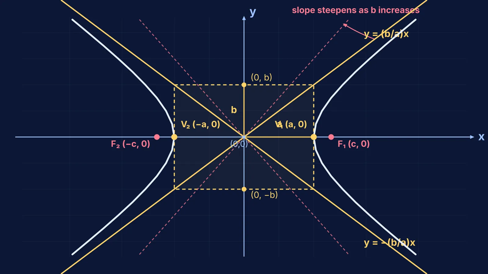
Finding asymptote equations depends on the orientation of the hyperbola's transverse axis. According to OpenStax Precalculus 2e, constructing a central rectangle provides the fastest path:
Identify the center: For unshifted standard equations, the center lies at (0, 0).
Identify transverse and conjugate axes: For x²/a² − y²/b² = 1, the transverse semi-axis length is a along the x-axis, and the conjugate semi-axis length is b along the y-axis.
Draw the central rectangle: Sketch a box centered at the origin with horizontal width 2a and vertical height 2b. The vertices lie on the box at (±a, 0), and co-vertices lie at (0, ±b).
Extend the diagonals: The asymptotes are the lines formed by extending the diagonals of this rectangle through the center.
For horizontal hyperbolas, the asymptotes are y = ±(b/a)x. For vertical hyperbolas y²/a² − x²/b² = 1, the asymptotes become y = ±(a/b)x. An algebraic shortcut consists of replacing the constant 1 with 0. Factoring x²/a² − y²/b² = 0 yields (x/a − y/b)(x/a + y/b) = 0, directly revealing both lines.
How does changing a and b turn the asymptote lines?
The slopes of the asymptotes depend on the ratio of the semi-axes. For a horizontal hyperbola, the upward slope is m = b/a. Because the asymptotes define the corridor where the hyperbola spreads, changing a and b turns these lines:
Increasing b relative to a: The central rectangle stretches vertically, increasing the slope b/a. The asymptotes steepen, causing the branches to open wider vertically.
Increasing a relative to b: The central rectangle widens horizontally, lowering the slope b/a toward zero. The asymptotes flatten, compressing the branches closer to the x-axis.
Equal axes (a = b): The equation simplifies to x² − y² = a², producing slopes m = ±1. The asymptotes meet at 90°, forming a rectangular hyperbola, as examined in our guide to hyperbola equations and asymptotes for JEE.
The opening angle between the two asymptotes is given by 2θ = 2 tan⁻¹(b/a).
Worked example: how do you graph x²/16 − y²/9 = 1 with asymptotes?
Following the central rectangle method from OpenStax Precalculus 2e, consider graphing x²/16 − y²/9 = 1 step by step:
Identify parameters: With a² = 16 and b² = 9, we have a = 4 and b = 3. The center is (0, 0).
Find vertices and co-vertices: Because x² is positive, the transverse axis is horizontal. Vertices are (−4, 0) and (4, 0); co-vertices are (0, −3) and (0, 3).
Calculate foci: With c = √(a² + b²) = √(16 + 9) = 5, the foci sit at (−5, 0) and (5, 0).
Write asymptote equations: Using slopes ±(b/a) = ±3/4, the asymptotes are y = (3/4)x and y = −(3/4)x.
Determine the angle: Each asymptote forms an angle θ = tan⁻¹(3/4) ≈ 36.87° with the x-axis, giving a full opening angle of 73.74°.
To sketch the graph, draw the 8 by 6 central rectangle, extend the dashed diagonals, and sweep the hyperbola branches outward from (±4, 0) along the asymptotes.
Why does active prediction improve coordinate geometry intuition?
Students often memorize asymptote formulas as isolated fractions, causing frequent mix-ups between b/a and a/b under exam pressure. Educational research by Carl E. Wieman, Wendy K. Adams, and Katherine K. Perkins found that interactive simulations deepen conceptual understanding when students predict outcomes before manipulating variables. Predicting an asymptote's tilt before testing it turns passive memorization into active reasoning.
When visualizing how parameter changes reshape conics, dynamic tools clarify the geometry. Fermi Simulation Lab provides interactive simulations for ideas that are easier to see than to read, allowing students to adjust semi-axes and observe asymptotes rotate. For structured practice with coordinate geometry derivations, Fermi Problem Library offers worked problems with a step-by-step solver that explains the reasoning rather than printing an answer. When students get stuck analyzing conic sections, Fermi's AI tutor teaches rather than answers, noticing where a student is stuck, drawing the figure, and checking understanding as it goes.


