On this page
Hardy-Weinberg is easier to believe once you have watched it fail. Below is one starting population, the prediction for it, and five spreadsheet runs that each break one condition. Make your prediction before each run; the surprises are where the learning happens.
What does Hardy-Weinberg equilibrium predict?
The mathematician G. H. Hardy set out the result in a two-page paper, Mendelian proportions in a mixed population, in Science in July 1908. The principle also carries the name of its co-discoverer, the German obstetrician Wilhelm Weinberg. The NCERT Class 12 Biology textbook states the principle simply: allele frequencies in a population are stable and constant from generation to generation (Chapter 6, section 6.7).
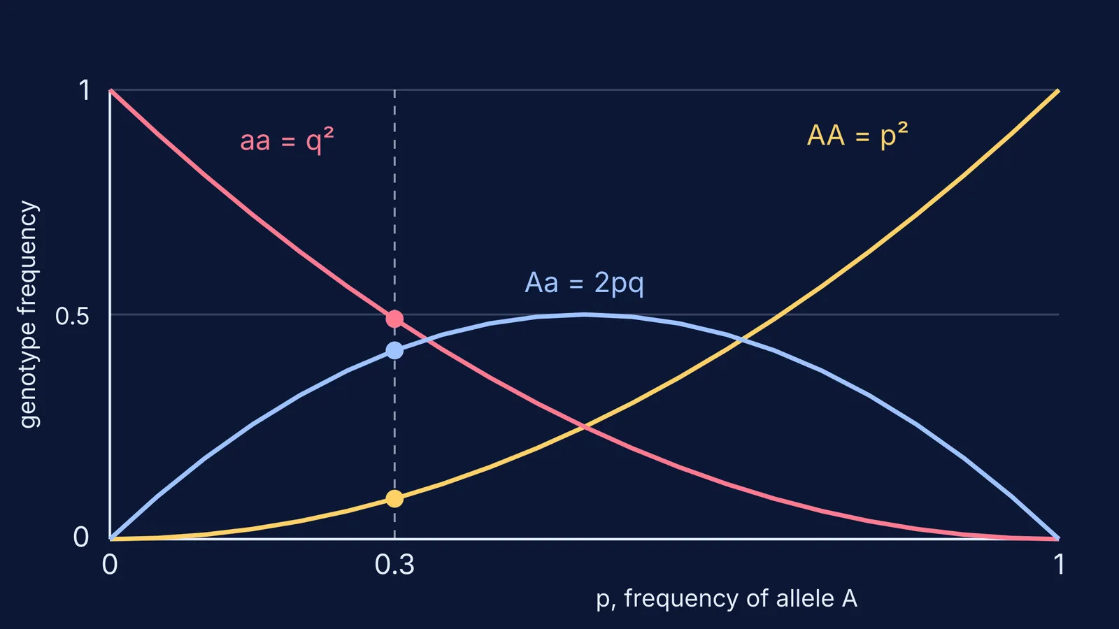
If p is the frequency of allele A and q the frequency of allele a, the genotype frequencies are AA = p², Aa = 2pq and aa = q², and p² + 2pq + q² = 1, the binomial expansion of (p + q)².
Worked prediction for p = 0.3, q = 0.7:
AA = 0.3 × 0.3 = 0.09
Aa = 2 × 0.3 × 0.7 = 0.42
aa = 0.7 × 0.7 = 0.49
In a population of 1,000 imaginary beetles, that is 90 AA, 420 Aa and 490 aa.
How do you simulate Hardy-Weinberg in a spreadsheet?
One row per generation is enough.
Column A: generation 0, 1, 2 and so on down to 50.
Column B: the allele frequency p. Type 0.3 in B2.
Columns C, D, E: =B2^2, =2*B2*(1-B2) and =(1-B2)^2 for AA, Aa and aa.
In B3, the next generation's p: =C2+D2/2. Copy everything down.
With nothing broken, p sits at 0.3 in every row. That flat line is the equilibrium. Now change only the B3 formula, one condition at a time.
What happens when you break each condition?
NCERT names five factors that affect Hardy-Weinberg equilibrium: gene migration or gene flow, genetic drift, mutation, genetic recombination and natural selection. The standard model also assumes a large population whose members choose mating partners at random. Here is what each break does, starting from p = 0.3. The numbers come from the formulas shown, so you can check them yourself.
Selection. Let aa leave only 80% as many offspring as the other genotypes: B3 = B2/(1-0.2*(1-B2)^2). p climbs 0.30, 0.333, 0.365, 0.397, 0.428 and reaches 0.458 after five generations.
Migration. Each generation, 5% of the population arrives from a group where p = 0.8: B3 = 0.95*B2+0.05*0.8. p passes 0.50 at generation 10 and 0.62 at generation 20, heading for 0.8.
Mutation. A turns into a at a rate of 1 in 100,000 per generation: B3 = B2*(1-0.00001). After 1,000 generations p has only fallen to 0.297. Mutation supplies new alleles but on its own moves frequencies very slowly.
Non-random mating. Let every individual self-fertilise for one generation. Heterozygotes halve from 0.42 to 0.21, AA rises to 0.195 and aa to 0.595, yet p is still exactly 0.3.
Recombination. This reshuffles which alleles of two or more genes travel together, so a one-gene sheet like this one cannot show it. Add a second gene if you want to try.
Why does a small population drift?
The equations above assume an infinitely large population. A real one samples its alleles each generation, and small samples wobble. In the spreadsheet, replace B3 with =BINOM.INV(2*N,B2,RAND())/(2*N), where N is the number of individuals (in Google Sheets, CRITBINOM does the same job). Press recalculate and the line jitters differently every time.
Population geneticists measure this loss with heterozygosity H, which shrinks by H/2N each generation and halves every 2N ln 2 generations. For 20 individuals that half-life is about 28 generations; for 1,000 it is about 1,386. After 100 generations a population of 20 keeps roughly 8% of its starting heterozygosity, against about 95% for 1,000.
The same source shows that a neutral allele's chance of eventually taking over equals its current frequency. So copy your drift column ten times with N = 20 and p = 0.3, run it for a few hundred generations, and count: on average about 3 of the 10 runs should end with A fixed and the rest with A lost. Our profile of Sewall Wright and genetic drift in small populations tells the story behind this idea.
How do you use this for revision?
Before each run, write three predictions on paper:
Does p change, or only the genotypes?
Which way does it move, and does it level off?
Is the change steady (selection, migration) or random (drift)?
Then run it and mark yourself. For the board and entrance-exam view of the same chapter, read our evolution guide covering natural selection and Hardy-Weinberg, and for the mathematician behind the equation, G. H. Hardy and his law of genetics.
If a term such as gene pool or fixation is still fuzzy, the Fermi Concept Library has a lesson for every concept in biology, each with its place in the map. For other ideas that are easier to see than to read, try the interactive simulations in the Fermi Simulation Lab.