

On this page
Reading that equipotentials are "perpendicular to field lines" is easy to forget. Drawing them yourself in a simulation is not. Below is a plan for the PhET browser simulation Charges and Fields, where you drop +1 nC and −1 nC charges and plot equipotentials with a voltage sensor. Write down a prediction before every click.
What is an equipotential line?
An equipotential line is a line along which the electric potential is constant; in three dimensions it becomes an equipotential surface, as OpenStax University Physics Volume 2 defines it.
The potential of a point charge is V = kq/r, with k = 8.99 × 10⁹ N·m²/C², and potentials from several charges simply add as numbers (OpenStax, section 7.3). V depends only on r, so a lone charge's equipotentials are circles in a 2D simulation.
For a +1 nC charge, kq = 8.99 V·m, so r = 8.99/V metres. The 40 V, 30 V, 20 V and 10 V lines sit at about 0.22 m, 0.30 m, 0.45 m and 0.90 m: equal voltage steps, growing gaps.
OpenStax compares equipotentials to contour lines on a hill map: where the slope is constant, the lines are evenly spaced. Crowded lines mean a steep potential and a strong field. Our guide to finding E from the slope of V turns that picture into E = −dV/dx.
How do you map equipotentials in the simulation?
Open Charges and Fields and drag one +1 nC charge to the middle of the screen.
Tick Electric Field, Voltage, Grid and Values.
Drag the voltage sensor to a point, read it, then use the sensor's button to plot the equipotential through that point. Plot four lines at equal voltage steps.
Add a −1 nC charge nearby to make a dipole, clear the old lines and plot again.
If you'd rather start from a ready-made set-up, the Fermi Simulation Lab has interactive simulations for the ideas that are easier to see than to read.
Why do field lines cross equipotentials at right angles?
Predict first: before you switch on the field arrows, sketch how they will sit against your circles.
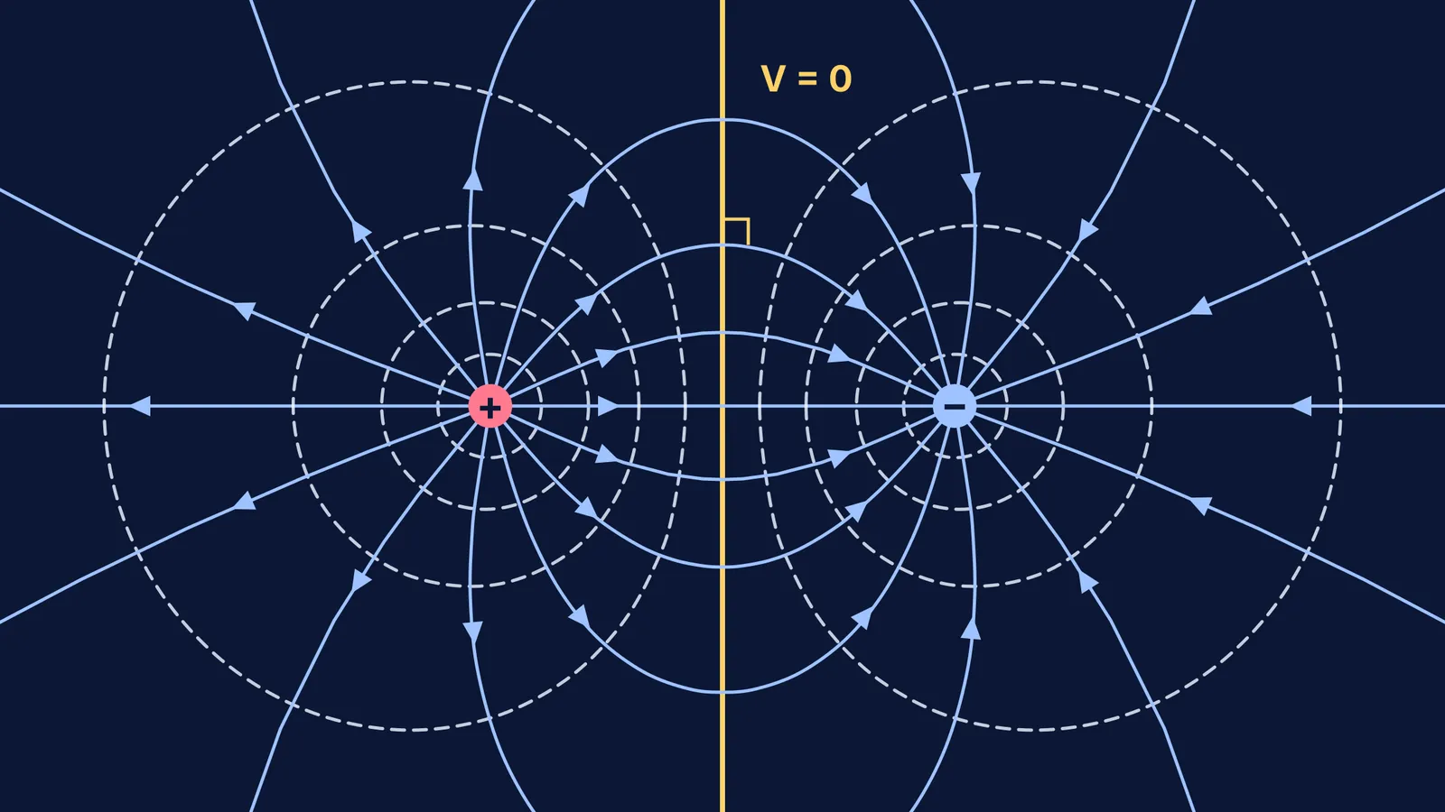
Then check: every field arrow crosses an equipotential at 90°, even where the dipole lines curve.
The reason is work. OpenStax states that equipotential lines are always perpendicular to electric field lines. The work done moving a charge q a small distance d is W = qEd cos θ. Along an equipotential ΔV = 0, so W = 0. Since neither q nor E is zero, cos θ must be zero, and θ = 90°.
Where is the potential zero for a dipole?
Predict first: with +1 nC and −1 nC on the screen, which points will read 0 V?
Then check. Drag the sensor along the perpendicular bisector of the two charges. It reads 0 V all the way, and the equipotential it plots is straight.
Every point on that perpendicular bisector is the same distance r from both charges, so kq/r − kq/r = 0. OpenStax describes this as the line where "the positive potential from the positive charge cancels the negative potential from the negative charge".
Worked example, using V = kq/r (OpenStax 7.3): put +1 nC and −1 nC 1.0 m apart. At a point between them, 0.25 m from the positive charge, V = 8.99 × (1/0.25 − 1/0.75) ≈ 24 V. At the midpoint, V = 8.99 × (2 − 2) = 0. At a point 0.25 m outside the positive charge on the same axis, V = 8.99 × (4 − 0.8) ≈ 29 V.
With unequal charges the zero points move; our guide on where the potential is zero near two charges does the algebra.
Why is no work done along an equipotential?
Predict first: you carry a +2 nC charge once round the 24 V line from the example. How much work does the field do?
The answer is zero. OpenStax gives W = −qΔV, and ΔV = 0 between any two points on the same equipotential. Work appears only when you cross lines. Move the same +2 nC charge from the 24 V point to the 0 V midpoint and the field does W = −(2 × 10⁻⁹ C)(0 − 24 V) ≈ 4.8 × 10⁻⁸ J.
Only the two end potentials enter that formula, so for work "along any path" from A to B, ignore the route.
What should you write down after the simulation?
One sketch per set-up: equipotentials dashed, field lines solid, arrows running from + to −.
The three rules in your own words, each with the line of algebra that proves it.
Sensor readings beside your hand calculations; if they disagree, check units.
The trap: V = 0 does not mean E = 0.
When you move on to dipole energy and torque, our guide to electric potential and dipoles picks up from here. If a step in the reasoning still feels shaky, Fermi's AI tutor can draw the figure, run the simulation and check your understanding as it goes.


