

On this page
If you cross two pea plants that are heterozygous for two traits—like seed shape and seed colour—you expect their offspring to show a 9:3:3:1 phenotypic ratio. But drawing a 16-box Punnett square on paper only shows you the mathematical probability. To see if real plants actually follow the rules, you need to grow hundreds of them and count every single seed.
Active learning makes a difference here. A major analysis of STEM education found that failure rates under traditional lecturing increase by 55% over the rates observed under active learning methods (Freeman et al., PNAS). Instead of just memorising the numbers from a textbook, you can use the Fermi Simulation Lab, which provides interactive simulations for the ideas that are easier to see than to read. You can cross virtual plants thousands of times in seconds and watch the 9:3:3:1 ratio emerge from the chaos of random chance.
What is a dihybrid cross?
A dihybrid cross tracks the inheritance of two different traits at the same time. In Gregor Mendel's classic experiment, he looked at pea shape (round or wrinkled) and pea colour (yellow or green). He wanted to know if inheriting a specific colour affected the chances of inheriting a specific shape.
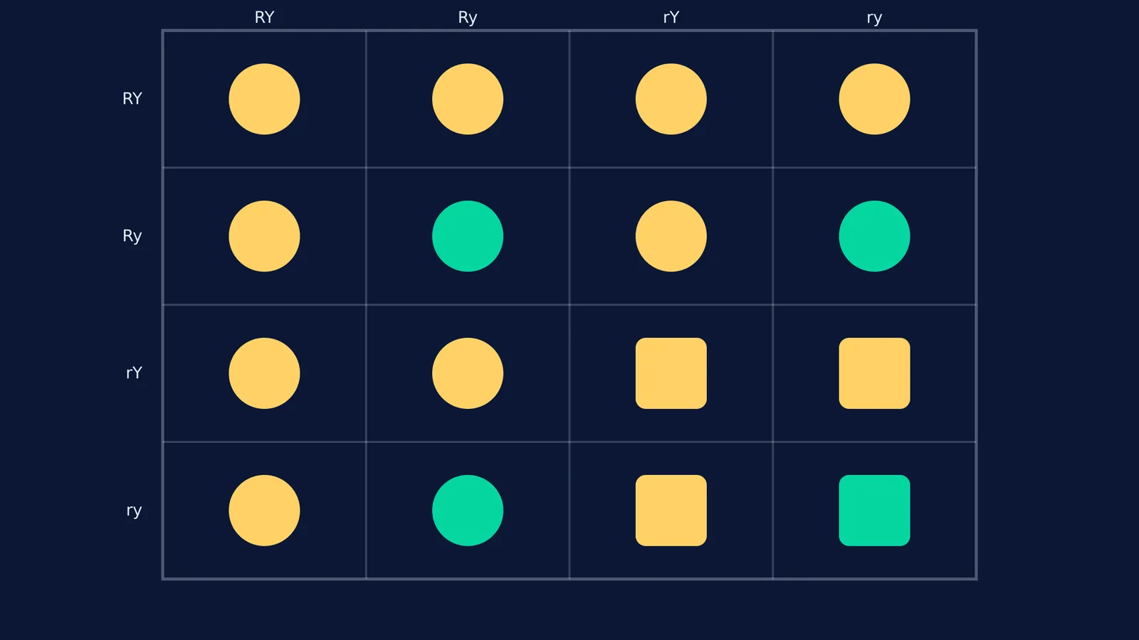
The parents in a standard dihybrid cross are heterozygous for both traits. If "R" is the dominant round allele, "r" is the recessive wrinkled allele, "Y" is the dominant yellow allele, and "y" is the recessive green allele, both parents have the genotype RrYy. To find an unknown genotype instead, you would use a test cross vs back cross, but here we start knowing exactly what the parents carry.
Where does the 9:3:3:1 ratio come from?
When you cross two RrYy parents, their alleles sort independently into gametes. This means a gamete carrying the "R" allele has an equal chance of carrying the "Y" or "y" allele. Because each trait follows a 3:1 dominant-to-recessive pattern when looked at on its own, multiplying the probabilities of the two traits gives you the combined ratio:
9/16 will have both dominant traits (round and yellow).
3/16 will have one dominant and one recessive trait (round and green).
3/16 will have the other dominant and recessive mix (wrinkled and yellow).
1/16 will have both recessive traits (wrinkled and green).
This mathematical spread is known as the law of independent assortment. It assumes the genes are on different chromosomes and do not interfere with each other, unlike complex Mendelian disorders where one gene can cause multiple downstream effects.
How did Mendel find the 9:3:3:1 ratio?
Mendel did not start with a 16-box Punnett square; he started with a garden. He manually pollinated pea plants, carefully tying bags over the flowers to prevent random insects from altering his results, and counted the seeds they produced.
In his F2 generation, Mendel collected exactly 556 seeds (Abbott & Fairbanks, 2016). He sorted them by hand and counted 315 round yellow, 108 round green, 101 wrinkled yellow, and 32 wrinkled green seeds. If you divide these numbers by 32, you get approximately 9.8 : 3.4 : 3.2 : 1. Mendel realised this was incredibly close to a perfect 9:3:3:1 ratio, proving that the traits were inherited independently. The slight variations were simply the result of statistical noise, just like flipping a coin might give you 52 heads and 48 tails.
Why are simulations better than static Punnett squares?
A Punnett square tells you what should happen on average, but biology is messy. If you grow exactly 16 pea plants in a greenhouse, you are very unlikely to get exactly 9 round yellow and 1 wrinkled green. You might get 11 round yellow and no wrinkled green at all.
This is where running a simulation changes how you learn. Rather than reading about Mendel's 556 seeds, you can simulate a genetic cross and generate 10, 100, or 10,000 offspring in a fraction of a second. If you are stuck on a genetics problem, Fermi's AI tutor can work out what you already know, build a plan for the session, and teach through it by running the simulation and checking understanding as it goes.
You will see that small sample sizes fluctuate wildly, but as the population grows, the results converge smoothly on the theoretical probability. This hands-on approach helps bridge the gap between abstract probability and real-world biology, giving you a clear mental model of how inheritance actually works.


