

On this page
You add water to a beaker of salt solution and the conductivity meter reading drops, yet textbooks say molar conductivity goes up. The idea is in NCERT's Class 12 chemistry, so it matters for CBSE and JEE Main. Below is a predict-then-check run you can do in a simulation or spreadsheet, using real numbers from the NCERT Class 12 Chemistry chapter on electrochemistry.
Why does conductivity fall but molar conductivity rise on dilution?
Conductivity (κ) measures how well one unit volume of solution conducts, and it always falls on dilution because there are fewer ions per unit volume (NCERT Class 12 Chemistry, Unit 2).
Molar conductivity, Λm = κ/c, is the conductance of the whole volume of solution that holds one mole of electrolyte. On dilution that volume grows faster than κ falls, so Λm rises for strong and weak electrolytes alike, according to the same NCERT chapter.
NCERT's table for KCl at 298.15 K shows both effects at once. Going from 1.000 to 0.010 mol L⁻¹, κ drops from 0.1113 to 0.00141 S cm⁻¹, while Λm climbs from 111.3 to 141.0 S cm² mol⁻¹.
Why does only the strong electrolyte give a straight line?
Set up two beakers: KCl, a strong electrolyte, and acetic acid (CH₃COOH), a weak one. Before you move the slider, write down your prediction. If you dilute each one 100 times, will Λm rise a little or a lot?
KCl is already fully split into ions, so dilution adds no new ones. Its Λm creeps up because the ions interfere with each other less as they spread out, a decrease in what the Wikipedia article on molar conductivity calls solute–solute interaction.
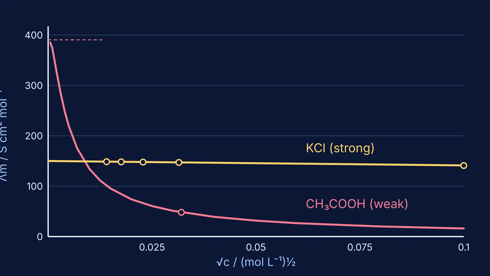
Kohlrausch's equation for strong electrolytes is Λm = Λ°m − A√c, so a plot of Λm against √c is a straight line with intercept Λ°m and slope −A (NCERT). In NCERT's Example 2.6, four very dilute KCl solutions give Λm between 148.61 and 147.09 S cm² mol⁻¹, and the fitted line gives Λ°m = 150.0 S cm² mol⁻¹ and A = 87.46.
Acetic acid behaves differently. NCERT explains that a weak electrolyte has a lower degree of dissociation at higher concentrations. On dilution, more molecules split into ions, so Λm rises steeply at low concentrations and Λ°m cannot be found by extrapolating to zero concentration.
What numbers should you expect to see?
NCERT's Example 2.9 gives 0.001028 mol L⁻¹ acetic acid a conductivity of κ = 4.95 × 10⁻⁵ S cm⁻¹, which gives Λm = 48.15 S cm² mol⁻¹, a degree of dissociation α = Λm/Λ°m = 0.1233, and Ka = 1.78 × 10⁻⁵ (NCERT).
We plugged that Ka and NCERT's Λ°m of 390.5 S cm² mol⁻¹ into NCERT's equation Ka = cα²/(1 − α) and solved it at other concentrations. Here is what we got:
At 0.01 mol L⁻¹, about 4% of the acid is ionised, and Λm is about 16 S cm² mol⁻¹.
At 0.0001 mol L⁻¹, about 34% is ionised, and Λm is about 134 S cm² mol⁻¹.
KCl over the same 100-fold dilution, using NCERT's fitted line, goes from about 141 to 149 S cm² mol⁻¹.
So the same dilution raises acetic acid's Λm about eight times but KCl's by only about 6%. If your simulation shows the reverse, check whether you are reading κ instead of Λm.
How do you find Λ°m for a weak electrolyte?
Since the curve cannot be extrapolated, use Kohlrausch's law of independent migration of ions: Λ°m is the sum of the limiting contributions of the cation and anion (NCERT). From NCERT's Table 2.4, λ°(H⁺) = 349.6 and λ°(CH₃COO⁻) = 40.9 S cm² mol⁻¹, which add to 390.5. NCERT's Example 2.8 reaches the same 390.5 from strong electrolytes alone: Λ°m(HCl) + Λ°m(CH₃COONa) − Λ°m(NaCl) = 425.9 + 91.0 − 126.4.
A predict-then-check plan for the simulation
Write your predictions first: which way κ and Λm will move for each electrolyte, and roughly how far.
Dilute KCl in steps (0.01, 0.001, 0.0001 mol L⁻¹), record Λm, and plot it against √c, not c.
Repeat with acetic acid on the same axes.
Draw a line through each set of points. Note where the KCl line meets the axis and why the acetic acid points refuse to sit on a line.
Work out α at each acetic acid point using Λ°m = 390.5, and check that Ka stays near 1.78 × 10⁻⁵.
Compare the results with your predictions and note what surprised you.
For ideas like this, the Fermi Simulation Lab has interactive simulations for ideas that are easier to see than to read. If the jump from κ to α still feels shaky, Fermi's AI tutor can work out what you already know and build a plan for the session.
For more practice, work through these molar conductivity and Kohlrausch's law examples, see how a cell constant turns measured resistance into conductivity, and read how J. C. Ghosh built a theory of strong electrolytes.


