

On this page
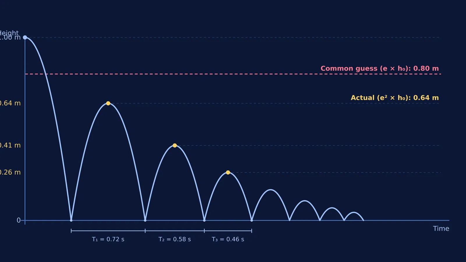
When physics students first encounter the coefficient of restitution, denoted by e, intuition frequently leads them astray. If a ball is dropped from a height of 1.00 m above a rigid floor with e = 0.8, the standard guess is that it will rebound to 80 cm, or 80% of its release height. It feels natural to assume that elasticity translates directly into recovered height (Cross, 2000).
In reality, the coefficient of restitution is defined as the ratio of relative separation speed to relative approach speed along the line of impact. In a classic investigation of colliding spheres in the *American Journal of Physics*, physicist Rod Cross emphasized that restitution measures velocity, not height or energy (Cross, 2000).
Just before impact, a ball falling from rest through drop height h₀ converts its gravitational potential energy into kinetic energy, reaching impact speed v₀ = √(2gh₀). Upon bouncing, it leaves the floor with upward velocity v₁ = e × v₀.
Because maximum rebound height h₁ depends quadratically on launch speed through the kinematic relation h₁ = v₁² / (2g), substituting v₁ = e × v₀ yields h₁ = (e × v₀)² / (2g) = e² × (v₀² / (2g)) = e² × h₀.
For e = 0.8, the rebound height factor is e² = 0.8² = 0.64. Dropping the ball from 1.00 m therefore produces a first bounce of only 0.64 m, or 64 cm (Cross, 2000). Because kinetic energy is proportional to velocity squared, retaining 80% of speed means the collision dissipates 36% of total mechanical energy on the very first impact.
How does height decrease after each consecutive bounce?
This quadratic scaling repeats on every rebound. When the ball falls back from height h₁, it strikes the floor with speed v₁ and rebounds at speed v₂ = e × v₁ = e² × v₀.
The second rebound height is therefore h₂ = e² × h₁ = e⁴ × h₀. Generalising to the nth rebound, the maximum height reached after n impacts is hₙ = e²ⁿ × h₀ (Cross, 2000).
For our ball dropped from h₀ = 1.00 m with restitution e = 0.8:
Bounce 1 reaches h₁ = 0.640 m (64.0 cm).
Bounce 2 reaches h₂ = 0.410 m (41.0 cm).
Bounce 3 reaches h₃ = 0.262 m (26.2 cm).
Bounce 4 reaches h₄ = 0.168 m (16.8 cm).
Bounce 5 reaches h₅ = 0.107 m (10.7 cm).
The rebound heights form a geometric progression with common ratio r = e² = 0.64. By the fifth impact, the ball rebounds to barely 10% of its initial release height, even though a restitution of 0.8 sounds quite springy (Cross, 2000).
In competitive exams like JEE Main, mechanics problems frequently test this distinction between speed and displacement. Combining the kinematic equations of vertical motion under gravity with momentum conservation principles in collisions and momentum problems prevents students from falling into linear decay assumptions.
Why do flight times between bounces scale with e instead of e²?
While peak heights decay by a factor of 0.64 on each bounce, the flight duration between impacts follows a different geometric ratio.
For a vertical bounce launched with upward speed vₙ, the ball takes time t_up = vₙ / g to reach its peak and an identical duration t_down = vₙ / g to return to the floor. The total time in the air between the nth impact and the (n+1)th impact is Tₙ = 2vₙ / g.
Because rebound speed scales linearly with restitution as vₙ = e × vₙ₋₁, the flight duration also scales linearly: Tₙ = e × Tₙ₋₁. Consecutive flight times form a geometric progression with common ratio e = 0.8, not e² = 0.64.
In 1977, physicist Alan D. Bernstein published an experiment in the *American Journal of Physics* showing that students can determine restitution simply by listening to the tempo of bouncing sounds (Bernstein, 1977). Because the acoustic delay between impacts equals Tₙ, the ratio of successive intervals directly gives e = Tₙ₊₁ / Tₙ.
Subsequent research confirmed that acoustic recording with ordinary microphones yields highly accurate measurements of both restitution and gravitational acceleration (Aguiar and Laudares, 2003). For an initial 1.00 m drop taking t₀ = √(2h₀/g) ≈ 0.452 s to strike the floor, the first bounce airborne time is T₁ = 2 × 0.8 × 0.452 s ≈ 0.723 s. The second bounce lasts T₂ = 0.8 × 0.723 s ≈ 0.578 s, and the third lasts T₃ = 0.8 × 0.578 s ≈ 0.463 s (Aguiar and Laudares, 2003).
What happens to the total distance and total time?
A classic puzzle asks whether an object that bounces infinitely many times must travel an infinite distance or take infinite time. Summing the geometric series resolves both questions.
The total vertical distance D consists of the initial drop h₀ plus twice each rebound height: D = h₀ + 2h₁ + 2h₂ + 2h₃ + ... Factoring out terms yields an infinite geometric series with first term e² and ratio e²: D = h₀ [1 + 2e² / (1 - e²)] = h₀ (1 + e²) / (1 - e²).
For h₀ = 1.00 m and e = 0.8, the numerator 1 + e² equals 1.64 and the denominator 1 - e² equals 0.36. The total distance traversed is 1.00 m × (1.64 / 0.36) ≈ 4.56 m before motion ceases (Cross, 2000).
The total time t_total until the ball stops bouncing combines the initial fall t₀ with all airborne intervals: t_total = t₀ + T₁ + T₂ + T₃ + ... Summing this geometric series gives t_total = t₀ [(1 + e) / (1 - e)].
For e = 0.8, the time multiplier (1 + 0.8) / (1 - 0.8) equals 1.8 / 0.2 = 9. The entire infinite cascade of bounces completes in exactly 9 times the initial drop time, or approximately 4.07 s for a 1.00 m drop (Bernstein, 1977).
How does active prediction sharpen your physical intuition?
Passively reading formulas rarely dislodges persistent misconceptions about velocity and height. In physics education research, Richard F. Gunstone and Richard T. White demonstrated that students must make an explicit, committed prediction before witnessing an event to trigger conceptual change (Gunstone and White, 1981).
This Predict-Observe-Explain (POE) approach encourages students to commit to a number, test it against empirical data, and reconcile the difference. Studies in science education found that multimedia and interactive simulations make POE tasks substantially more effective by giving immediate visual feedback on physical variables (Kearney et al., 2001).
As shown in research comparing simulations vs static diagrams, adjusting physical parameters interactively helps learners connect abstract energy graphs with physical motion.
To build genuine intuition for dynamic mechanics, the Fermi Simulation Lab offers interactive simulations for ideas that are easier to see than to read. When tackling multi-stage numericals, the Fermi Problem Library provides worked problems with a step-by-step solver that explains the reasoning rather than printing an answer.


