

On this page
In calculus, finding the exact area under a curve by computing a definite integral is not always possible. Many functions simply do not have an antiderivative that can be written in terms of standard algebraic or trigonometric expressions. When an exact mathematical solution escapes us, we turn to numerical methods to find highly accurate approximations. Among these techniques, Simpson's rule is arguably the most famous and widely taught in high schools and universities worldwide. However, the name attached to this powerful mathematical tool hides a complex history that spans more than a century and involves several brilliant minds.
What is Simpson's rule?
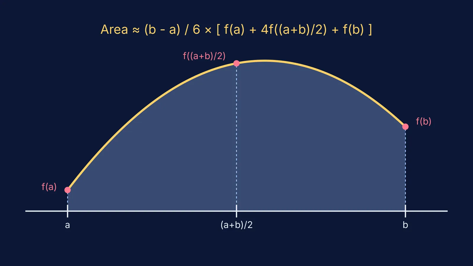
If you have a continuous curve and need to find the area under it between two points on the x-axis, say a and b, Simpson's rule replaces the complex curve with a simple quadratic polynomial (a parabola). Because the area under a parabola is easy to calculate, this swap gives a remarkably accurate estimate of the true area.
The basic formula, known as Simpson's 1/3 rule, requires evaluating the function at three specific points: the start (a), the midpoint ((a+b)/2), and the end (b). The formula is: Area ≈ (b − a)/6 × [f(a) + 4f((a+b)/2) + f(b)].
For larger intervals, we use the composite rule. You divide the total area into an even number of strips, apply the basic rule to consecutive pairs of strips, and sum the results. This technique forms the backbone of computational integration in physics and engineering. If you are working through calculus assignments and struggle to set up these bounds, the Fermi Problem Library has a step-by-step solver that explains the reasoning rather than just printing an answer.
Who invented Simpson's rule?
The history of Simpson's rule reveals that the method was discovered, used, and published long before Thomas Simpson was born.
In his 1615 published work *Nova stereometria doliorum vinariorum* (New Stereometry of Wine Barrels), Johannes Kepler sought a reliable way to calculate the volume of wine barrels. He had noticed that wine merchants in Austria were using inaccurate methods to price their barrels based on rudimentary measurements, and he decided to find a rigorous geometric solution. Because of his discovery, the integration technique is still commonly known in Germany as Kepler's barrel rule (*Keplersche Fassregel*).
Decades later, in 1639, Bonaventura Cavalieri, an Italian mathematician and student of Galileo, explored similar ideas regarding indivisibles and areas. By the 1660s, the Scottish mathematician James Gregory had formally stated the rule (MacTutor). Even Sir Isaac Newton developed the formula independently during his foundational work on calculus.
Who was Thomas Simpson?
Thomas Simpson (1710–1761) was a British mathematician whose path to academic recognition was entirely unconventional (MacTutor). Born to a weaver in Leicestershire, Simpson received very little formal schooling as a child and initially worked in his father's trade.
A self-taught mathematician, his early years were turbulent. According to the MacTutor History of Mathematics archive, Simpson had a brief career in astrology and had to flee his hometown for Derby after an incident where he reportedly frightened a client by pretending to raise a devil. He eventually moved to London, where he supported his family by weaving silk during the day and teaching mathematics in the city's coffee houses at night.
In 1743, Simpson published *Mathematical Dissertations on a Variety of Physical and Analytical Subjects* (Wikipedia). This widely read textbook included the rule for numerical integration that now bears his name. Simpson was entirely transparent about his sources, openly acknowledging that he had learned the technique from Isaac Newton. However, because Simpson was a gifted teacher and his textbooks were remarkably clear, accessible, and widely distributed, generations of students learned the technique from him and began associating the method entirely with his name.
If you find yourself stuck on complex calculus histories or struggling to connect the dots in your own studies, Fermi's AI tutor can work out what you already know and build a plan for the session.
How can you master numerical integration?
When tackling numerical integration problems in your exams, having a solid routine prevents careless arithmetic mistakes. Simpson's rule requires careful bookkeeping of your values, especially when you are pressed for time.
Here is a practical checklist for applying the composite rule effectively:
Check the strips: Ensure the number of subintervals (n) is an even number. Simpson's 1/3 rule only works when you pair up strips, meaning n must be even.
Find the step size: Calculate the width of each strip as h = (b − a) / n. Write this number down clearly at the top of your page.
Tabulate your values: Create a table with two columns. In the first column, write your x values starting from a and adding h each time until you reach b. In the second column, calculate the corresponding f(x) values.
Apply the weights: Remember the alternating multiplier pattern: 1, 4, 2, 4, 2, ... 4, 1. The first and last function values are multiplied by 1, the odd-indexed terms by 4, and the even-indexed terms by 2.
Do the final multiplication: Sum all the weighted terms and multiply the total by h / 3.
By organising your work into a clear table, you minimise the chance of miskeying a number into your calculator. To see how these structural principles apply to standard algebraic integrals, you might review the properties of definite integrals or explore the substitution method for integrating 1/(a + b cos x).


