

On this page
When Gilbert N. Lewis introduced the electron-pair bond in 1916, he gave chemistry an indispensable bookkeeping system. Lewis structures showed which atoms shared electrons and which held lone pairs, but they were flat diagrams. They offered no way to deduce whether a molecule was linear, pyramidal, or bent. Linus Pauling introduced orbital hybridisation in 1931, yet calculating angles from wavefunctions was difficult, and simple valence bond models could not explain why molecules with identical coordination numbers had noticeably different bond angles.
Why did chemists need a geometric model of bonding?
In 1940, British chemists Nevil Sidgwick and Herbert Powell took an important step in their Royal Society Bakerian Lecture, *Stereochemical types and valency groups*. They proposed that the spatial arrangement of bonds around a central atom is determined by the total number of electron pairs in its valence shell. Electron pairs repel one another and adopt shapes that maximise their distance: two pairs align linearly at 180°, three form an equilateral triangle at 120°, four form a tetrahedron at 109.5°, five form a trigonal bipyramid, and six form an octahedron at 90°.
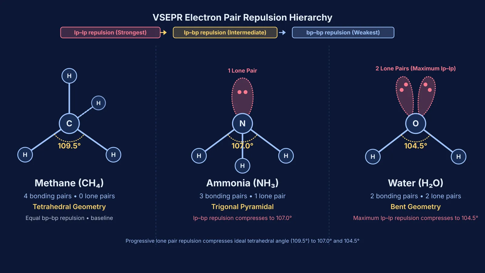
Yet Sidgwick and Powell treated all electron pairs as equal. If all pairs repelled identically, every four-pair molecule would have a 109.5° bond angle. Instead, experimental spectroscopy showed that methane (CH₄) formed a 109.5° angle (109° 28'), ammonia (NH₃) contracted to 107.0° (recorded as 106° 7' in early reports), and water (H₂O) closed to 104.5° (104° 27'), as catalogued in Gillespie and Nyholm's *Inorganic stereochemistry*. Chemists needed a rule that accounted for the differing spatial sizes of electron pairs.
How did Gillespie and Nyholm turn electron repulsion into VSEPR theory?
At University College London in 1957, Ronald Gillespie and Ronald Nyholm solved this problem in *Inorganic stereochemistry*, published in *Quarterly Reviews, Chemical Society*. They realised that electron pairs occupy different volumes of space.
A bonding pair is shared between two positive nuclei, confining its electron cloud between the atoms. A non-bonding lone pair is attracted to only one nucleus. Without a second positive charge to constrain it, the lone pair spreads wider, occupying greater volume near the central atom.
From this spatial asymmetry, Gillespie and Nyholm established the repulsion hierarchy of Valence Shell Electron Pair Repulsion (VSEPR) theory:
Lone pair – lone pair (lp–lp) repulsion is strongest.
Lone pair – bonding pair (lp–bp) repulsion is intermediate.
Bonding pair – bonding pair (bp–bp) repulsion is weakest.
Why do lone pairs compress bond angles?
This hierarchy explained molecular distortions across the periodic table, as Gillespie and Nyholm detailed in *Inorganic stereochemistry*. In methane, four bonding pairs experience identical repulsion, preserving the 109.5° tetrahedral angle. In ammonia, one lone pair exerts stronger lp–bp repulsion on the three N–H pairs, compressing the bond angle to 107.0°. In water, two lone pairs repel each other with maximum lp–lp force, squeezing the O–H bonds to 104.5°.
Ronald Gillespie later highlighted the quantum mechanical foundation of this model in the *Journal of Chemical Education*. While taught as electrostatic repulsion, the primary force keeping electron pairs apart is the Pauli exclusion principle, which prevents electrons of identical spin from occupying the same space.
For students exploring these geometry changes, the Fermi Simulation Lab offers interactive simulations for ideas that are easier to see than to read.
How can you predict any molecule's shape with Gillespie-Nyholm rules?
Gillespie and Nyholm systematised their model into a practical four-step procedure in *Inorganic stereochemistry* for chemistry curricula and competitive examinations such as JEE Main, JEE Advanced, and NEET-UG. To predict molecular shapes using VSEPR in four steps:
Count valence electrons: Find the central atom's valence electrons, adjusting for ionic charge.
Find the steric number: Add bonded atoms (sigma bonds) and central lone pairs. Multiple bonds count as one domain.
Determine electron geometry: Map domains to standard geometries (linear for 2, trigonal planar for 3, tetrahedral for 4, trigonal bipyramidal for 5, octahedral for 6).
Position lone pairs to minimise repulsion: In trigonal bipyramidal geometry, place lone pairs equatorially to minimise 90° interactions. In octahedral geometry, place two lone pairs trans at 180°.
Consider chlorine trifluoride (ClF₃), an example common in the shapes of interhalogen compounds like ClF₃ and BrF₅. Chlorine has 7 valence electrons, sharing 3 with fluorine and retaining 2 lone pairs. With a steric number of 5, the electron geometry is trigonal bipyramidal. Placing both lone pairs in equatorial positions minimises lp–lp repulsion, yielding a bent T-shape with an axial-equatorial angle compressed slightly below 90° to 87.5°.
When working through complex geometries such as see-saw SF₄ or square planar XeF₄, the Fermi Problem Library offers worked problems with step-by-step hints and solutions that explain the underlying reasoning.


