On this page
When water flows through a pipe, blood courses through your veins, or air rushes past a wing, the fluid's speed and pressure at every point change from moment to moment. For nearly two centuries, physicists, meteorologists and engineers have relied on the Navier-Stokes equations to describe this motion and predict how a fluid will behave in the real world.
Derived independently by French engineer Claude-Louis Navier and British physicist George Gabriel Stokes in the 19th century, these equations essentially apply Newton's second law of motion—that force equals mass times acceleration—to a fluid. While they capture the underlying physics of viscous, real-world fluids perfectly, they are famously frustrating and difficult to solve. The equations contain a nonlinear convective term that makes the fluid's acceleration depend on the velocity itself. Physically, this nonlinear term describes how a flow can fold over itself and twist into chaotic eddies, vortices and full-blown turbulence.
Mathematically, this same term can theoretically cause the equations to "blow up." This means that the calculated velocity of the fluid could become infinite in a finite amount of time, a situation that makes absolutely no physical sense in the real world. Finding out exactly when and how this happens—and whether the three-dimensional equations always have smooth, predictable solutions—remains one of the great unsolved problems in mathematics, carrying a million-dollar Millennium Prize from the Clay Mathematics Institute.
But Olga Ladyzhenskaya made foundational steps toward taming these equations and bringing mathematical rigour to fluid dynamics.
What did Olga Ladyzhenskaya prove?
Born in Russia on 7 March 1922, Olga Ladyzhenskaya spent much of her career tackling the mathematics of fluid dynamics. She faced severe early challenges because her father was executed during Stalinist purges, which initially barred her from entering university. Despite this, she went on to become one of the most influential mathematicians of her era.
When Ladyzhenskaya first began working on the Navier-Stokes equations, she was unaware of similar research being done independently by mathematicians like Jean Leray and Eberhard Hopf.
In the late 1950s and into the 1960s, she obtained key results regarding the existence and uniqueness of solutions for these equations. She also became the "L" in the celebrated LBB (Ladyzhenskaya-Babuška-Brezzi) condition, which arises in mixed finite element discretizations of the Stokes and Navier-Stokes equations. She consolidated her foundational proofs in her 1961 book, *The Mathematical Theory of Viscous Incompressible Flow*, which quickly became a classic text for mathematicians and physicists worldwide.
How do computers use her work?
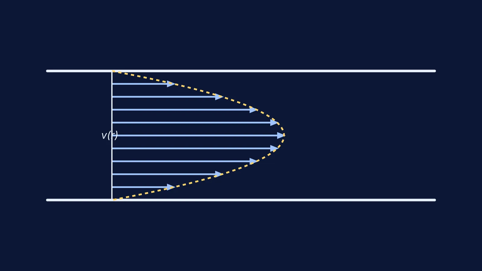
Beyond her theoretical proofs, Ladyzhenskaya was a pioneer in translating abstract mathematics into practical calculations. Engineers rarely solve the Navier-Stokes equations by hand, because exact analytical solutions only exist for the simplest cases—like steady flow through a straight pipe. Instead, they use a technique called finite difference methods, where space and time are chopped into a grid, and computers calculate the flow step by step.
Ladyzhenskaya provided the first rigorous proof that these finite difference methods actually converge to the true physical solution for the Navier-Stokes equations. This was a monumental achievement because it meant numerical approximations could be trusted. Her proofs laid the solid mathematical foundation for modern computational fluid dynamics (CFD). Today, every time an aerospace engineer simulates the aerodynamics of a new car design, or a meteorologist runs a massive weather forecast model on a supercomputer to predict a storm's path, they rely on the mathematical stability guarantees that she helped establish.
A checklist for fluid mechanics students
When you encounter problems involving fluid motion in your physics or engineering courses, keeping the physical meaning of the math clear is crucial. Here is a quick checklist to help you set up your equations correctly:
Identify the dimensions: Are you solving a one-dimensional, two-dimensional or three-dimensional problem? The mathematics changes significantly for each, and choosing the simplest dimension that captures the physics will save you time.
Check the fluid properties: Is the fluid viscous (like syrup or engine oil) or ideal (with no internal friction)? The Navier-Stokes equations handle viscosity, while the simpler Euler equations describe ideal flow.
Look for symmetries: Can you assume the flow is steady (meaning it does not change with time) or incompressible (meaning it has a constant density)? These assumptions make the equations much easier to solve and are often true for low-speed liquid flows.
If you are studying fluid mechanics: pressure, buoyancy and Bernoulli mistakes to avoid, seeing the flow can help. The Fermi Simulation Lab provides interactive simulations for the ideas that are easier to see than to read. You can also explore how other scientists approached the field, like Roddam Narasimha and turbulence in fluid flow.