

On this page
Why did early transatlantic telegraph signals suffer severe delay?
In the 1850s, overland telegraphs carried Morse pulses almost instantaneously. Suspended wires had negligible capacitance to ground, allowing electrical signals to travel along the wire near the speed of light.
Submarine cables behaved differently. When engineers attempted to bridge the 3,000-kilometre Atlantic Ocean, signals suffered severe "retardation"—pulses slowed down and arrived as indistinct murmurs. Michael Faraday and Latimer Clark noticed this sluggish response on underground lines, prompting mathematician George Gabriel Stokes to consult William Thomson (later Lord Kelvin) in October 1854 (Thomson, 1855).
Thomson identified the mechanism: an underwater cable is a giant capacitor. The copper conductor is insulated by gutta-percha and submerged in conductive seawater connected to ground. When an operator keyed a signal in Ireland, the battery had to charge the continuous dielectric sheath before a readable voltage appeared in Newfoundland (Thomson, 1855).
How does Thomson's law of squares govern cable diffusion?
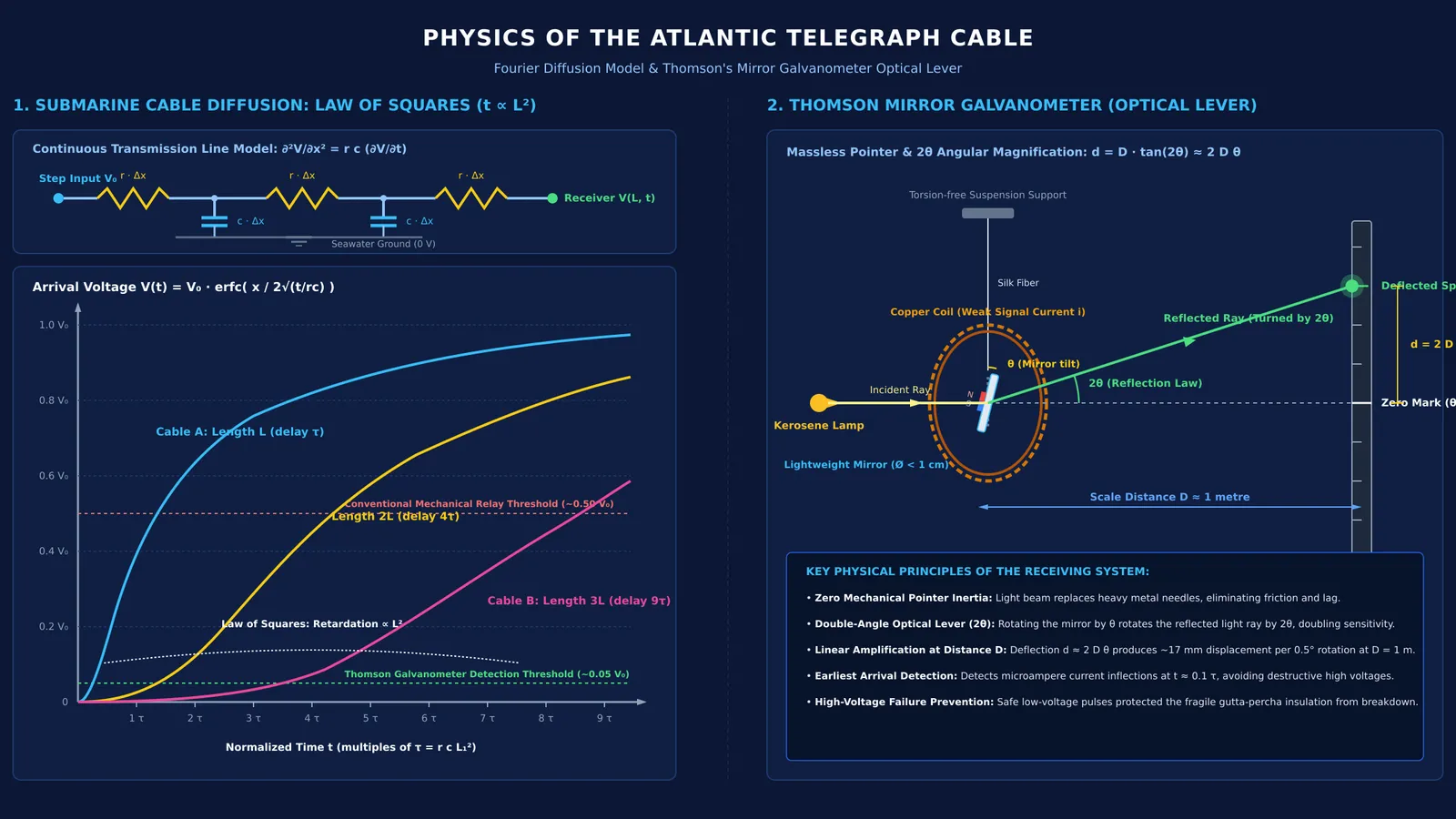
In his 1855 Royal Society paper, "On the Theory of the Electric Telegraph", Thomson showed that submarine signals do not obey the wave equation (Thomson, 1855). Because telegraph frequencies were low and cable capacitance was vast, inductive effects were negligible. The voltage V at distance x and time t obeys Joseph Fourier's heat diffusion equation:
∂²V/∂x² = r c (∂V/∂t)
Here, r is conductor resistance per unit length and c is capacitance per unit length. Because an undersea cable forms concentric conductors separated by insulation, finding c requires the logarithmic formula for a cylindrical capacitor.
From this equation, Thomson derived his Law of Squares: signal delay scales with the square of cable length, proportional to r c L² (Thomson, 1855). Doubling the length quadruples the delay; ten times the length yields a 100-fold retardation.
The Atlantic Telegraph Company's chief electrician, Edward Whitehouse, rejected Thomson's theory (Britannica). Whitehouse insisted electricity could be forced through with higher voltage. In 1858, he applied induction coils generating up to 2,000 volts, puncturing the gutta-percha insulation and destroying the cable after only a few weeks (ETHW).
How did the mirror galvanometer make faint pulses readable?
Thomson realized high voltage was destructive. The receiving end saw a slow, S-shaped diffusion curve rather than a sharp step. The solution was detecting the earliest microampere current inflection without waiting for the cable to fully charge.
To read these faint signals, Thomson patented the mirror galvanometer in 1858 (Britannica). Conventional galvanometers relied on heavy metal needles whose inertia and pivot friction required large currents. Thomson replaced the physical pointer with a massless optical lever.
He attached tiny magnets to the back of a lightweight mirror suspended by a silk fiber inside a coil. A lamp projected light onto the mirror, reflecting a spot onto a scale roughly 1 metre away.
Because the reflected ray turns through twice the mirror's deflection angle (2θ), an angular rotation of 0.5 degrees moved the light spot by roughly 17 millimetres on a 1-metre scale. The instrument proved far more sensitive than conventional needle receivers (ETHW). On July 27, 1866, the steamship Great Eastern landed a permanent cable at Heart's Content, Newfoundland, establishing an enduring transatlantic link via Thomson's receiving instruments (IEEE Milestones). Thomson was knighted for the achievement in 1866 (Britannica).
How do you calculate the square-law cable delay?
To see why Thomson's Law of Squares dictated cable design, compare a 300-kilometre coastal line (L₁) with a 3,000-kilometre transatlantic line (L₂) of equal cross-section (Thomson, 1855):
Resistance per metre (r): Core radius a = 1.4 millimetres (area A ≈ 6.16 × 10⁻⁶ m²), copper resistivity ρ = 1.72 × 10⁻⁸ Ω·m. r = ρ / A ≈ 2.79 × 10⁻³ Ω/m.
Capacitance per metre (c): Gutta-percha insulation outer radius b = 4.6 millimetres, relative permittivity ε_r = 3.2. c = 2π ε₀ ε_r / ln(b/a) ≈ 1.50 × 10⁻¹⁰ F/m.
Diffusion constant (r c): r c = (2.79 × 10⁻³ Ω/m) × (1.50 × 10⁻¹⁰ F/m) ≈ 4.19 × 10⁻¹³ s/m².
Diffusion time constant (τ = r c L²): For Cable A (3.0 × 10⁵ m), τ₁ ≈ 0.038 seconds (38 milliseconds). For Cable B (3.0 × 10⁶ m), τ₂ ≈ 3.77 seconds.
Retardation ratio: τ₂ / τ₁ = (L₂ / L₁)² = 10² = 100.
A 38-millisecond delay on a 300-kilometre line is imperceptible, but a 3.77-second time constant across 3,000 kilometres severely smears consecutive Morse pulses. Cable engineers solved this by thickening the copper core to reduce r and using Thomson's galvanometer to detect the earliest current arrivals.
What does Kelvin's cable teach about electrical modeling?
Thomson's cable analysis founded transmission line theory. Oliver Heaviside generalized it into the telegrapher's equations, and Edith Clarke applied distributed parameters to power transmission lines. Long-distance links eventually shifted from copper conductors to light pulses through Narinder Singh Kapany's optical fibres.
For students studying RC circuits in JEE physics, Thomson's model demonstrates how diffusion equations solve practical engineering bottlenecks.
If you find distributed parameters difficult to visualise, the Fermi Simulation Lab provides interactive simulations for the ideas that are easier to see than to read. To practice multi-step RC circuit transients, the Fermi Problem Library offers worked problems with a step-by-step solver that explains the reasoning rather than printing an answer. For a complete syllabus map linking electrostatics, current electricity, and capacitance, explore the Fermi Concept Library, where every concept in physics has its own lesson and its place in the map.


