

On this page
Why did early artificial intelligence struggle with uncertainty?
In the 1970s and early 1980s, computer scientists believed human thought could be reduced to rules of formal logic. Expert systems relied on chains of deterministic IF-THEN statements. But as John McCarthy and the origins of artificial intelligence revealed, real-world knowledge is never clean or complete. Sensors produce noisy measurements, medical symptoms point to multiple diseases, and everyday human judgements rely on plausible hunches rather than rigid mathematical proofs.
When researchers attempted to capture uncertainty using traditional probability, they hit a combinatorial wall. Describing thirty related binary variables without independence assumptions requires a joint probability distribution with 2³⁰ − 1—more than 1.07 billion—numerical probabilities. No computer of the era had the memory to store that table, and no expert could supply the numbers. As Judea Pearl documented in his landmark 1986 paper in *Artificial Intelligence*90072-x), machines needed a structured way to exploit conditional independence.
How do Bayesian networks let computers update belief?
Pearl’s solution was the Bayesian network: a directed acyclic graph where nodes represent random variables and arrows represent direct statistical or causal dependencies. Instead of memorising every combination of events, a Bayesian network factorises the overall joint probability into local conditional probabilities: each variable depends solely on its immediate parents.
If thirty variables are arranged so that each node has at most two parents, the system requires fewer than 120 conditional probabilities instead of one billion. In his 1986 paper in *Artificial Intelligence*90072-x), Pearl introduced the belief propagation algorithm, which allows nodes to update their probabilities by passing messages locally across the graph. Just as Andrey Markov's memoryless chains simplified sequential processes, Pearl’s networks turned intractable probability spaces into efficient, linear-time calculations. By combining graph theory with Bayes' theorem and conditional probability, computers could finally update their beliefs in real time as fresh evidence arrived.
What is Judea Pearl's Ladder of Causation?
Although Bayesian networks mastered uncertain associations, Pearl realised they possessed a blind spot. A network can tell you that a falling barometer correlates with rain, but it cannot tell you whether tampering with the barometer will cause a storm. In his 2000 book *Causality: Models, Reasoning, and Inference* and his 2019 review in *Communications of the ACM*, Pearl formalised this insight into the "Ladder of Causation", which classifies cognitive reasoning into three distinct levels:
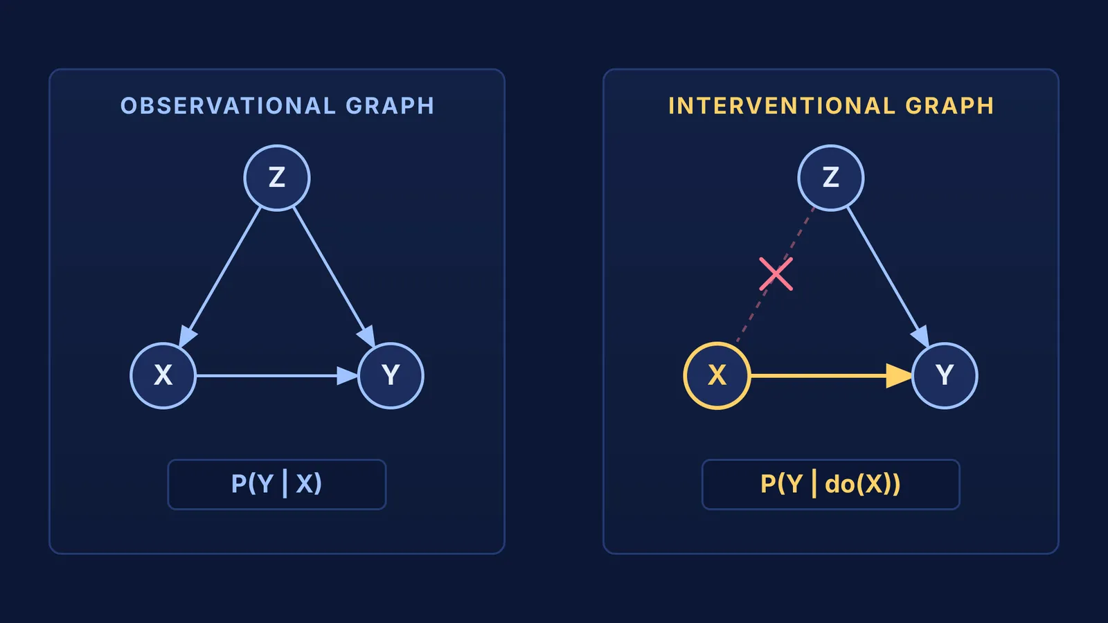
Rung 1: Association (Seeing). This is the realm of passive observation and conventional machine learning. It asks: "If I observe event X, how likely is event Y?" It is computed using standard conditional probability P(Y | X).
Rung 2: Intervention (Doing). This level asks: "What will happen to Y if we actively do X?" Pearl invented the "do-operator", written P(Y | do(X)), to represent deliberate action. In a 1995 paper in *Biometrika*, he proved the rules of "do-calculus", showing how to predict interventional effects by mathematically severing incoming arrows to the intervened variable.
Rung 3: Counterfactuals (Imagining). This highest level asks retrospection: "What would have happened if we had acted differently?" It underpins concepts of credit, blame, and scientific explanation.
How does conditional independence explain away alternate causes?
One of Pearl’s most celebrated insights, detailed in his treatise *Causality: Models, Reasoning, and Inference*, is the behaviour of "colliders" (v-structures), where two independent causes converge on a shared effect (A → C ← B). In these structures, two completely unrelated events become conditionally dependent once their shared consequence is known.
Consider a practical diagnostic example. Suppose a student solves a challenging physics problem and arrives at an incorrect final numerical answer (event E = 1). Two independent explanations exist:
A conceptual misunderstanding of the physics law (event M), with prior probability P(M) = 0.20.
A careless minus-sign error in the algebra (event S), with prior probability P(S) = 0.30.
Assuming either mistake alone causes an incorrect result, the prior probability of an error is 1 − (1 − 0.20)(1 − 0.30) = 0.44 (44%). Observing that the final answer is wrong raises both probabilities: P(M | E = 1) jumps from 20% to 0.20 / 0.44 ≈ 45.5%, while P(S | E = 1) rises to 0.30 / 0.44 ≈ 68.2%. But when the tutor inspects the student's notebook and spots a clear minus-sign error (S = 1), that arithmetic slip fully accounts for the mistake. The probability of a conceptual failure P(M | E = 1, S = 1) immediately collapses back to its baseline of 20.0%. Finding the calculation slip "explains away" the wrong answer. Pearl’s graph mathematics proved that conditioning on a common effect creates an informational bridge between independent causes.
How does causal reasoning shape modern AI tutoring?
Human teachers use this diagnostic logic instinctively. When a student struggles with a problem, an effective tutor does not simply register a failure; it isolates whether the error came from a missing prerequisite, a computational slip, or an incorrect intuition.
Modern educational technology applies these same structural principles. The Fermi Problem Library provides worked problems with a step-by-step solver that explains the reasoning rather than printing an answer, making it easy to isolate the exact step where an error occurred. When you want to trace how core ideas depend on one another, the Fermi Concept Library maps every concept across mathematics and computing, placing each topic in its wider relational framework so you can build strong foundations from the ground up.


