

On this page
The Newton-Raphson method is a powerful mathematical tool for finding the roots of equations. But despite its hyphenated name, Isaac Newton and Joseph Raphson never collaborated, and neither of them wrote down the formula students use today.
How did Isaac Newton solve equations?
Isaac Newton first described a method for approximating roots in a manuscript written around 1669, De analysi per aequationes numero terminorum infinitas, though it was not published until 1711 Wikipedia. He later expanded on it in his 1671 work Method of Fluxions, which also remained unpublished until 1736. His original approach was quite different from the modern technique.
Newton applied his logic exclusively to polynomials. Instead of a single, repeating formula, he used a long, algebraic substitution process. To correct an initial guess, he created an entirely new polynomial, solved it for a small correction value while ignoring higher-power terms, and added that back to his guess. He then repeated the process by creating yet another polynomial for the next correction.
While mathematically sound, Newton's process was tedious and prone to algebraic errors. Curiously, he did not use the calculus concepts of differentiating expressions that he was developing around the same time. His root-finding remained a purely algebraic exercise.
What did Joseph Raphson publish in 1690?
Joseph Raphson published a simplified root-finding method in his 1690 book Analysis Aequationum Universalis Wikipedia. This publication occurred decades before Newton's early manuscripts on the topic saw print.
Raphson realised that Newton's method of generating new polynomials for every step was unnecessary. Instead, he extracted the corrections directly from the original equation. Raphson's method was an iterative process of successive approximations, meaning the exact same mathematical operation could be applied repeatedly to hone in on the root. This made the calculation significantly easier to perform by hand.
Because his book was widely read while Newton's papers were still locked away in private study, the mathematical community largely learned the iterative technique from Raphson. John Wallis had published an earlier account of Newton's algebraic method in 1685, but Raphson's simpler presentation is what mathematicians actually adopted and used.
Who added the derivative to the Newton-Raphson formula?
The modern Newton-Raphson formula is xₙ₊₁ = xₙ - f(xₙ)/f'(xₙ). Despite the name, neither Newton nor Raphson included the derivative f'(x) in their work. Both relied on algebra rather than the new rules of calculus.
Thomas Simpson published the modern calculus-based version of the method in 1740 Wikipedia. By introducing the fluxion (the derivative), Simpson eliminated the need for algebraic approximations entirely. He also applied the technique to general nonlinear equations, extending it far beyond the simple polynomials that Newton and Raphson had studied. Simpson even generalised the method to handle systems of multiple equations and optimization problems.
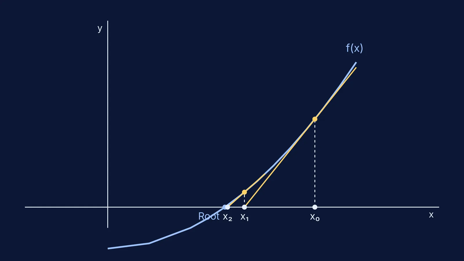
Later textbooks formally adopted the term "Newton-Raphson method" to honour both Newton's foundational idea and Raphson's iterative refinement. The modern method visually corresponds to drawing a tangent line to a curve and finding where it intersects the axis. If you are finding its roots by counting intersections of two sketched curves, you get a rough visual estimate. The Newton-Raphson method takes that estimate and hones it to high precision using the curve's exact slope.
How do you use the Newton-Raphson method?
The iterative nature of the modern formula makes it incredibly fast, often doubling the number of correct decimal places with each step Wikipedia. To solve x² - 2 = 0 (which finds the square root of 2):
Identify the function: f(x) = x² - 2
Find the derivative: f'(x) = 2x
Choose a starting guess, such as x₀ = 1.5.
Calculate the first iteration, x₁:
x₁ = 1.5 - (1.5² - 2) / (2 × 1.5) x₁ = 1.5 - (2.25 - 2) / 3 x₁ = 1.5 - 0.25 / 3 ≈ 1.4167
Use x₁ to find the next iteration, x₂:
x₂ = 1.4167 - (1.4167² - 2) / (2 × 1.4167) ≈ 1.4142
Within just two steps, the method yields an approximation accurate to four decimal places. When practicing iterative calculus topics for exams, getting stuck on the mechanics or losing track of decimal places is common. The Fermi Problem Library has worked problems with a step-by-step solver that explains the reasoning rather than printing an answer, helping you see exactly where an algebraic mistake happened. Working through these iterations by hand builds a strong intuition for how rates of change pinpoint exact values, an idea championed by early calculus pioneers like Guillaume de l'Hôpital. By understanding the history, you can appreciate how a tedious algebraic chore evolved into one of the most elegant tools in mathematics.


