On this page
In the 1930s, long-distance telephone networks were struggling with distortion and instability. The engineers at Bell Labs needed a way to build stable feedback amplifiers that would not break into spontaneous oscillation (or "singing") when component values drifted over time or due to temperature changes.
Hendrik Wade Bode (1905–1982) solved this problem in 1938 by introducing a graphical method to analyse system stability using frequency response. His invention, now universally known as the Bode plot, remains a cornerstone of modern control theory and electronics engineering. By turning complex transfer functions into simple geometric sketches, Bode gave engineers the tools they needed to design robust feedback systems.
Who was Hendrik Bode?
Born in Madison, Wisconsin, Bode was a child prodigy who graduated from high school at the age of 14. He went on to receive a bachelor's degree in mathematics from Ohio State University in 1924, followed by a master's degree in 1926. He joined Bell Labs immediately after his master's degree and spent over 40 years shaping the telecommunications industry, later completing a PhD in physics from Columbia University.
His work went far beyond telephone lines. Like Nicholas Callan and his induction coil, Bode’s mathematical innovations transformed practical electrical engineering. During World War II, Bode applied his control theory methods to anti-aircraft artillery. He served on the National Defense Research Committee (NDRC) and helped develop the automatic Director systems that used radar to track and destroy fast-moving targets. Winston Churchill specifically requested these automated gun units during the London Blitz to counter the German V-1 flying bombs.
The system proved extraordinarily effective. Combining the Director T-10 with microwave radar and proximity fuses, the automated guns shot down 1,629 V-1 flying bombs aimed at London in the summer of 1944. This remarkable achievement cemented his legacy not just as a mathematician, but as an engineer who solved some of the most critical and time-sensitive problems of his generation. His expertise in control systems laid the groundwork for modern robotics and aerospace navigation.
If you are studying control systems and cannot figure out where to begin, Fermi's AI tutor can work out what you already know and build a plan for the session, so you sit down to a clear next step instead of a blank page.
What is a Bode plot?
A Bode plot consists of two separate graphs that share a logarithmic horizontal axis for frequency. This logarithmic scale is essential because it allows engineers to display a massive range of frequencies—from hertz to gigahertz—on a single, readable chart. By expanding the lower frequencies and compressing the higher ones, the plot reveals the system's behaviour across different scales of operation.
Magnitude plot: This shows the system's gain (how much it amplifies or attenuates the input signal), measured in decibels (dB). Using decibels means that when you cascade multiple components, you can simply add their gains together rather than multiplying them.
Phase plot: This shows the phase shift between the input and output signals, measured in degrees. Like the magnitude in decibels, the phase shifts of cascaded components also simply add together, which greatly simplifies the overall analysis of complex networks.
When analysing complex circuits, visualizing these changes is often easier than working through the algebra. The Fermi Simulation Lab offers interactive simulations for the ideas that are easier to see than to read, such as the relationship between node potentials and frequency in an oscillating circuit.
How to draw a straight-line Bode plot?
Before digital computers, plotting exact points for a complex transfer function was tedious. Bode's great insight was that you could approximate the true, curved frequency response using straight-line asymptotes. This technique reduced a daunting computational task to a quick geometric exercise.
In control theory, the roots of the denominator of a transfer function are called "poles", and the roots of the numerator are called "zeros". Each pole or zero acts at a specific corner frequency (or break frequency), changing the slope of the response.
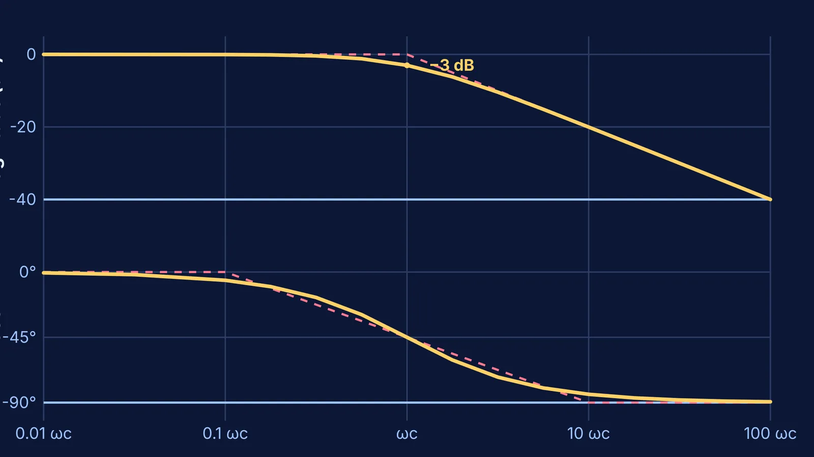
Here are the rules for drawing the asymptotic Bode plot of a simple low-pass filter, which has a single pole at a corner frequency of ωc:
Magnitude: The gain starts flat at 0 dB for low frequencies. At the corner frequency ωc, the asymptote breaks downward, falling at a steady rate of −20 dB per decade (a decade is a factor of 10 in frequency). The true curve smoothly follows these lines, dipping exactly −3 dB below the straight-line intersection at the corner.
Phase: The phase shift starts at 0°. A decade before the corner frequency, the phase begins to drop at −45° per decade. At exactly ωc, the phase is −45°. The phase stops dropping a decade after the corner, settling permanently at −90°.
By adding these simple straight lines together, engineers can quickly sketch the combined response of systems with multiple poles and zeros. This makes it possible to visually determine a system's gain margin and phase margin, turning the difficult task of stability analysis into a matter of geometry rather than complex arithmetic.