

On this page
Why did agricultural field trials need statistical blueprints?
In the early twentieth century, agricultural research faced a stubborn problem. Agronomists testing crop varieties or fertilisers observed wide yield variations across adjacent plots, even with identical seeds. Soil fertility, moisture, and drainage change across mere metres. In an unstructured field, spatial gradients easily swamped treatment effects or created misleading advantages for inferior varieties, a challenge directly tied to Liebig's law of the minimum for crop yield.
Ronald Fisher had demonstrated the mathematics of analysis of variance at Rothamsted Experimental Station in England, but field practitioners lacked practical blueprints for laying out trials. Gertrude Mary Cox (1900–1978), who earned the first Master of Science degree in statistics awarded by Iowa State College in 1931 under George Snedecor, recognized that scientists were wasting entire planting seasons collecting uninterpretable data. In her 1950 paper The Function of Designs in Experiments, Cox emphasised that statistical architecture cannot wait until harvest. If an experiment lacks a structured layout before planting, no retrospective analysis can rescue it from confounding bias.
How did Gertrude Cox turn experimental design into a working science?
In 1940, North Carolina State College sought to establish a Department of Experimental Statistics. When university president Frank Graham solicited recommendations from George Snedecor, Snedecor supplied a list of male candidates with a famous footnote: if the university would consider a woman, he recommended Gertrude Cox. The university appointed Cox in late 1940, and she established the Department of Experimental Statistics in 1941 as its first female professor and department head, as documented by the NC State Department of Statistics History and her records in the Gertrude Mary Cox Papers.
Cox quickly established North Carolina as an international hub for statistics. In 1944, she established the Institute of Statistics of the Consolidated University of North Carolina, describing its structure in her 1950 paper The Organization and Functions of the Institute of Statistics of the University of North Carolina. In 1946, she recruited Harold Hotelling to Chapel Hill to lead theoretical statistics, while she directed applied experimental consulting at Raleigh.
Her landmark contribution came in 1950 with the textbook *Experimental Designs*, co-authored with William G. Cochran. Published by John Wiley & Sons, the comprehensive manual became the standard reference across biology and agriculture. Rather than focusing solely on theoretical proofs, Cochran and Cox provided concrete, numbered combinatorial plans for randomized blocks, Latin squares, split-plot layouts, and lattice designs. In 1949, Cox became the first woman elected to the International Statistical Institute, and in 1956, she served as President of the American Statistical Association. In her presidential address, published in 1957 as Statistical Frontiers, Cox urged researchers to act as active explorers rather than passive tourists, designing trials that isolate true signals from background noise.
How does blocking isolate nuisance variance?
The mathematical engine of Cox's methodology is the partitioning of variance. When evaluating treatments, total variation reflects both genuine treatment effects and background experimental error. In an unblocked design, spatial field gradients directly inflate the residual error sum of squares.
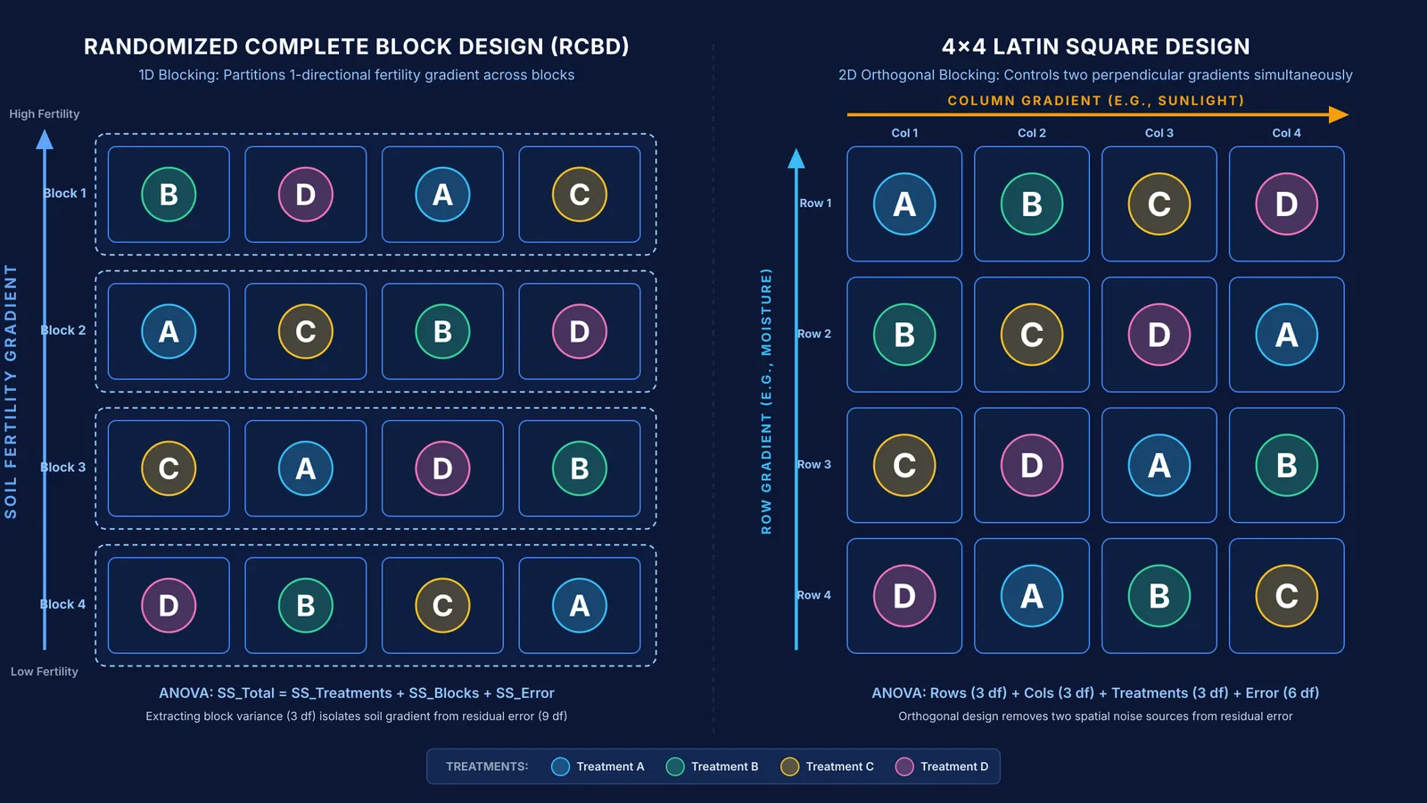
Cox's Randomized Complete Block Design groups experimental units into blocks perpendicular to the gradient. Total sum of squares is partitioned as:
SS_Total = SS_Treatments + SS_Blocks + SS_Error
By measuring and extracting the variance between blocks (SS_Blocks), residual error shrinks. Because the F-statistic compares treatment variance to error variance (F = MS_Treatments / MS_Error), a smaller denominator sharpens sensitivity to real treatment differences. This logic connects directly to calculating mean and variance.
For students observing how varying parameters shifts statistical distributions, the Fermi Simulation Lab provides interactive simulations for ideas that are easier to see than to read.
Which experimental layout should you choose for a trial?
In her 1950 survey A Survey of Types of Experimental Designs, Gertrude Cox categorized practical field layouts by matching design structures to the geometry of known confounding variations:
Completely Randomized Design (CRD): Use when units are fully homogeneous, such as well-mixed liquid cultures in identical test tubes.
Randomized Complete Block Design (RCBD): Use when one directional gradient exists, such as a slope or lighting gradient. Each treatment appears once per block.
Latin Square Design: Use when two orthogonal gradients operate simultaneously, such as row-wise moisture and column-wise sunlight. Each treatment appears once per row and once per column.
Incomplete Block Design: Use when testing many treatments (such as 25 crop hybrids) where complete blocks would be too large to remain homogeneous.
Consider a worked comparison of degrees of freedom (df) for 4 treatments replicated 4 times across 16 total plots:
Unblocked layout (CRD): Treatments have 3 df; residual error absorbs 12 df. Uncontrolled soil fertility inflates the error term, reducing test power.
One-dimensional blocking (RCBD): Treatments have 3 df, blocks take 3 df, and error retains 9 df. Removing block variation sharpens treatment comparisons.
Two-dimensional orthogonal blocking (4 × 4 Latin Square): Rows take 3 df, columns take 3 df, treatments take 3 df, and error retains 6 df, eliminating two independent environmental gradients.
Before running hypothesis tests, researchers often inspect raw data distributions with John Tukey's visual tools for inspecting distributions. When working through analysis of variance calculations, the Fermi Problem Library offers worked problems with a step-by-step solver that explains the reasoning rather than printing an answer.


