

On this page
Every Class 12 mathematics student learns the basics of linear programming, sketching intersecting lines to find a feasible region and hunting for the maximum or minimum value at its vertices. The mathematical foundation for this was laid by George Dantzig, who published the simplex method in 1947.
While quadratic word problems usually ask you to find a single correct value, linear programming asks you to find the absolute best value out of an infinite number of possibilities within a defined area.
What was Dantzig's famous homework mistake?
In 1939, while studying for his doctorate at UC Berkeley, George Dantzig arrived late to a statistics lecture taught by Jerzy Neyman. He saw two problems written on the blackboard and, assuming they were the week's homework, copied them down.
Dantzig worked on the problems, finding them slightly more difficult than usual, but he handed in his solutions a few days later. Six weeks later, Neyman excitedly informed a shocked Dantzig that the equations were not homework at all. They were actually two famous unsolved problems in statistics. Because Dantzig did not know the problems were supposedly impossible, he approached them with a positive mindset and cracked them. When Dantzig later asked about a thesis topic, Neyman told him to wrap the two problems in a binder and he would accept them as his thesis.
This persistence is crucial for tackling difficult subjects. Fermi's AI tutor works out what you already know and builds a plan for the session, holding a line of reasoning across a whole session to teach you through it.
What is linear programming?
During World War II, the military needed a way to plan logistics, calculating how to allocate troops, fuel, and supplies efficiently. Dantzig formulated these complex problems, a method that remained a military secret until 1947.
Linear programming is a mathematical method for determining the best outcome in a model where requirements are represented by linear relationships. It consists of three main parts:
The objective function: The quantity you want to maximise (like profit) or minimise (like cost).
The constraints: The limits on your resources, written as linear inequalities (e.g., 2x + y ≤ 100).
The feasible region: The area on a graph where all constraints overlap and hold true.
If you struggle with interpreting the graphical representation of these constraints, the Fermi Concept Library has every concept in mathematics, each with its own lesson and its place in the map, to help you visualise the regions.
How does the simplex method work?
For a textbook problem with only two variables (x and y), you can easily draw the lines on a graph and check the corners. But real-world resource problems have hundreds or thousands of variables. Finding the best assignment of 70 people to 70 jobs involves more possible combinations than there are particles in the universe.
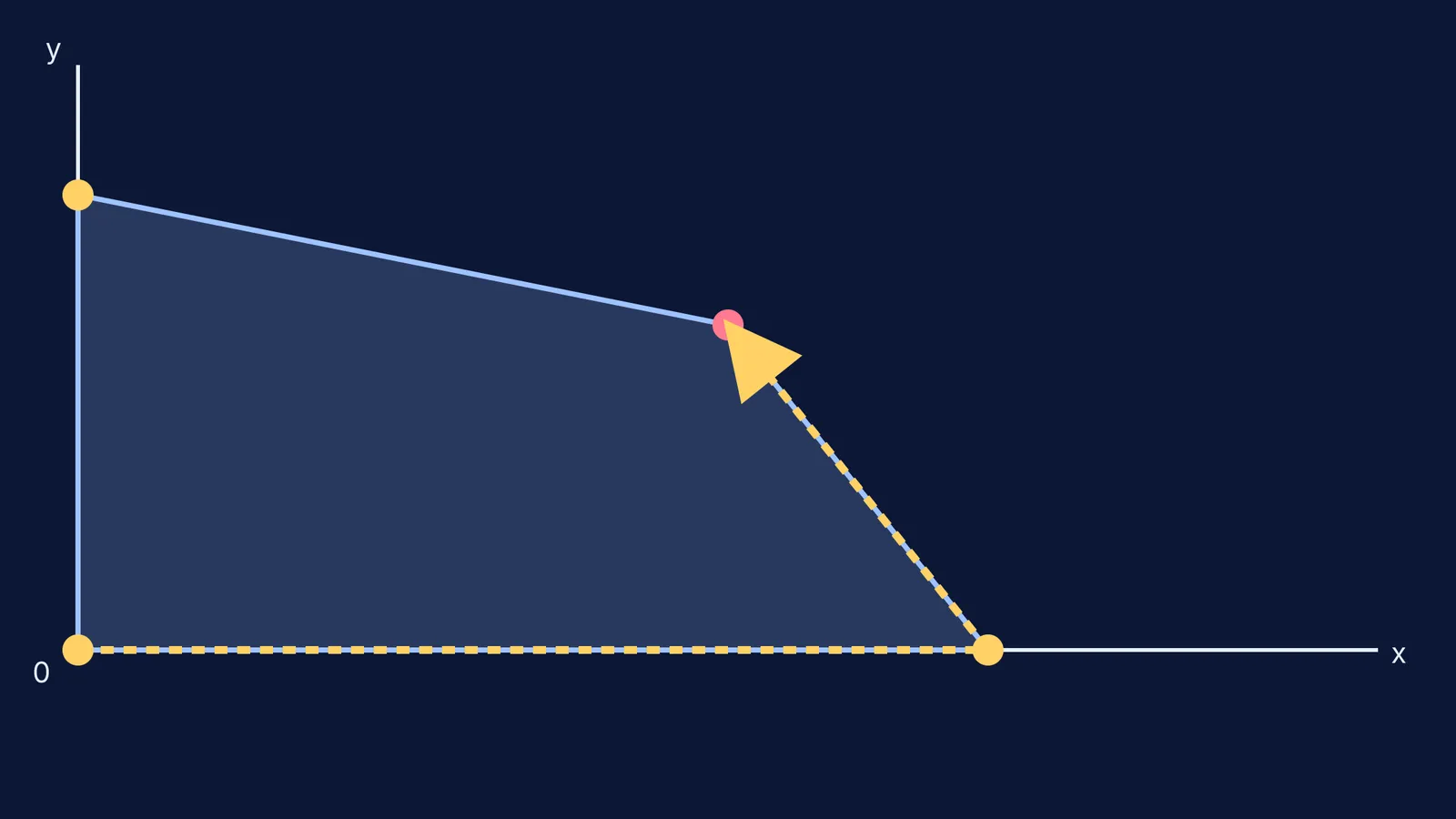
Dantzig's genius was the simplex method algorithm. Instead of checking every possible point inside the multi-dimensional shape, the algorithm only moves along the edges from one vertex to an adjacent vertex. At each step, it guarantees that the objective function improves, stopping immediately when it reaches the peak.
Just as you might find roots by curve intersections to solve polynomial equations, linear programming requires finding the intersections of straight boundary lines to locate these crucial vertices.
When you solve linear programming word problems, it is easy to set up the wrong equations from the start. The Fermi Problem Library has worked problems with a step-by-step solver that explains the reasoning rather than printing an answer.
How do you solve linear programming in Class 12?
To tackle linear programming questions in your Class 12 board exams, follow this reliable routine:
Define your variables: Clearly write down what x and y represent in the real world.
Write the objective function: Express the ultimate goal as Z = ax + by.
List the constraints: Convert the word problem into inequalities. Do not forget the non-negative constraints (x ≥ 0, y ≥ 0), as you cannot have negative resources.
Plot the lines: Find the x and y intercepts for each boundary equation to graph them quickly.
Shade the feasible region: Test the origin (0,0) to see which side of each line satisfies the inequality.
Find the vertices: Solve the intersecting equations simultaneously to find the exact coordinates of the corners.
Evaluate: Plug each vertex coordinate into your objective function Z. The highest value is your maximum; the lowest is your minimum.


