On this page
On 9 October 1986, the journal Nature published a four-page paper called Learning representations by back-propagating errors. Its authors were David Rumelhart, Geoffrey Hinton and Ronald Williams. It showed how a network could train its hidden layers, using the chain rule from Class 12 calculus over and over.
What did the 1986 backpropagation paper show?
The paper's abstract describes backpropagation as "a new learning procedure" for "networks of neurone-like units". The procedure "repeatedly adjusts the weights of the connections in the network so as to minimize a measure of the difference between the actual output vector of the net and the desired output vector."
The key result is about the hidden units. In the authors' words, internal "hidden" units "come to represent important features of the task domain". Nobody tells those units what to look for. The abstract says this ability to create useful new features is what sets backpropagation apart from "earlier, simpler methods such as the perceptron-convergence procedure".
The idea of shrinking a squared error is old. Legendre published it for fitting data in 1805, as we explain in our post on Adrien-Marie Legendre and the method of least squares. What the 1986 paper made clear was how to do it for a network with hidden layers in between, and what those layers then learn.
Why did hidden layers need the chain rule?
When the output is wrong, it is easy to see how the last weight affected the error. A hidden weight changes the hidden unit, which changes the output, which changes the error: a function inside a function inside a function.
The chain rule handles this. If E depends on y, y depends on h, and h depends on w, then dE/dw = (dE/dy) × (dy/dh) × (dh/dw). Backpropagation works out these factors from the output end first and reuses each one on the way back, so every weight gets its share of the blame in one backward pass.
How does backpropagation work, step by step?
Here is the smallest network that still has a hidden layer. Work it on paper alongside us. Input x = 2, hidden unit h = w1 × x, output y = w2 × h, target t = 2. The error is E = (1/2)(y - t)^2. Start with w1 = 0.5 and w2 = 3. Real networks add a squashing function; the chain rule still works.
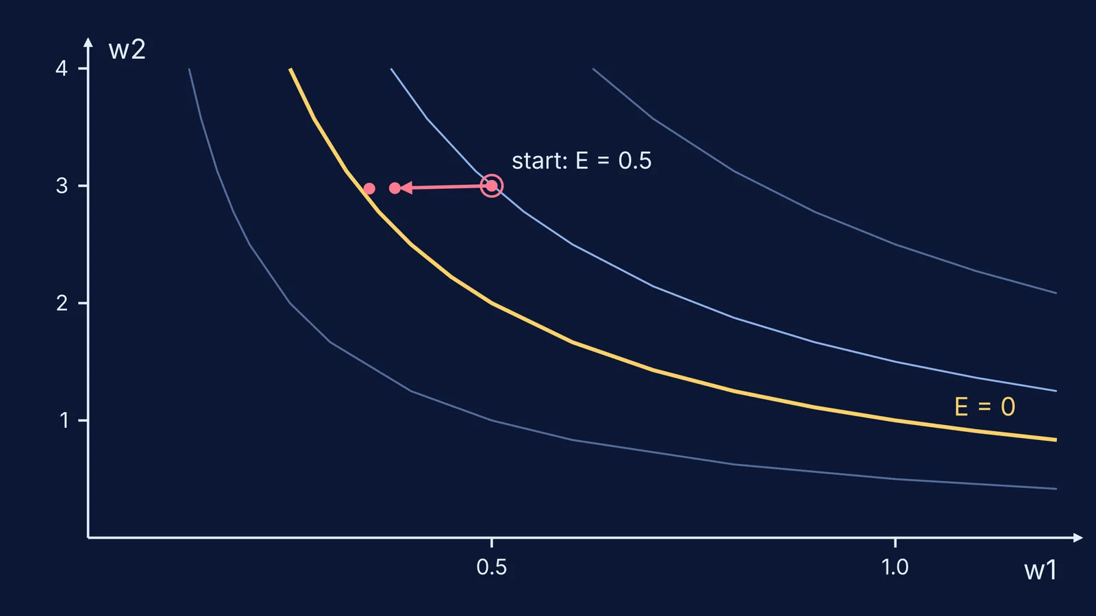
Forward pass: h = 0.5 × 2 = 1, then y = 3 × 1 = 3, so E = (1/2)(3 - 2)^2 = 0.5.
Start at the output: dE/dy = y - t = 1.
Last weight: dE/dw2 = (dE/dy) × h = 1 × 1 = 1.
Pass the error back to the hidden unit: dE/dh = (dE/dy) × w2 = 1 × 3 = 3.
Hidden weight: dE/dw1 = (dE/dh) × x = 3 × 2 = 6.
Update with a small step size of 0.02: w2 becomes 3 - 0.02 × 1 = 2.98, and w1 becomes 0.5 - 0.02 × 6 = 0.38.
Check: h = 0.76, y = 2.98 × 0.76 = 2.2648, so E = (1/2)(0.2648)^2, about 0.035.
One backward pass and update cut the error from 0.5 to about 0.035. The hidden weight got the bigger push because the chain rule showed its derivative was 6. A real network repeats the same steps, with far more weights and layers.
Why does a 1986 calculus idea still matter today?
The 2024 Nobel Prize in Physics was awarded jointly to John Hopfield and Geoffrey Hinton "for foundational discoveries and inventions that enable machine learning with artificial neural networks". The field had come a long way since the early ideas we trace in John McCarthy, the Dartmouth proposal and the birth of AI.
The 1986 paper did not appear from nowhere. Its reference list on Crossref cites Rosenblatt's 1961 book Principles of Neurodynamics, Minsky and Papert's 1969 book Perceptrons and a 1985 paper by Yann Le Cun.
How can you practise the calculus behind backpropagation?
Use this checklist on any composite function:
Write the chain of dependencies in words first: E depends on y, y on h, h on w.
Find each small derivative on its own before multiplying.
Work from the outside in, and reuse what you have already found.
Check by changing one weight a little and seeing if E moves as your derivative predicted.
If the chain rule itself feels shaky, the Fermi Concept Library has a lesson for every concept in mathematics, each with its place in the map, so you can see what differentiation builds on. For calculus in physics, see our guide to calculus for JEE physics.
When you get stuck partway through a derivative, the Fermi Problem Library has worked problems with a step-by-step solver that explains the reasoning rather than printing an answer.