

On this page
In 1905 the Austrian physicist Egon von Schweidler made a prediction at a radiology congress in Liège. If each radioactive atom breaks up purely by chance, the count from a steady source cannot be perfectly smooth. It has to jitter by an amount probability can predict. That jitter shows the smooth decay curve in your textbook is built out of randomness.
Who was Egon von Schweidler?
Schweidler was born in Vienna on 10 February 1873 and died on 12 February 1948, according to his entry in the Neue Deutsche Biographie. That entry calls his paper on the fluctuations of radioactive decay, printed in 1906, foundational, because it proved for the first time that decay is statistical. He gave the talk in Liège in 1905; the congress proceedings came out the next year.
What did Schweidler argue in 1905?
The clearest record comes from those who later tested him. In their 1910 paper on alpha particles, Ernest Rutherford and Hans Geiger wrote: "The magnitude of the probability variations in the number of α particles was first drawn attention to by E. v. Schweidler." They cite his Liège talk of 1905.
His result, in their words, was that the average error from the mean number of alpha particles is √(N·t), where N is the number emitted per second and t is the counting interval (Rutherford and Geiger, 1910). So if you expect to count 100 particles, the actual count will typically be off by about 10.
Picture two models. In one, each atom is a clock set to go off at a fixed age. In the other, each atom holds a lottery ticket, and every instant carries the same small chance. Schweidler's jitter belongs to the lottery.
Why does random decay give an exponential law and a half-life?
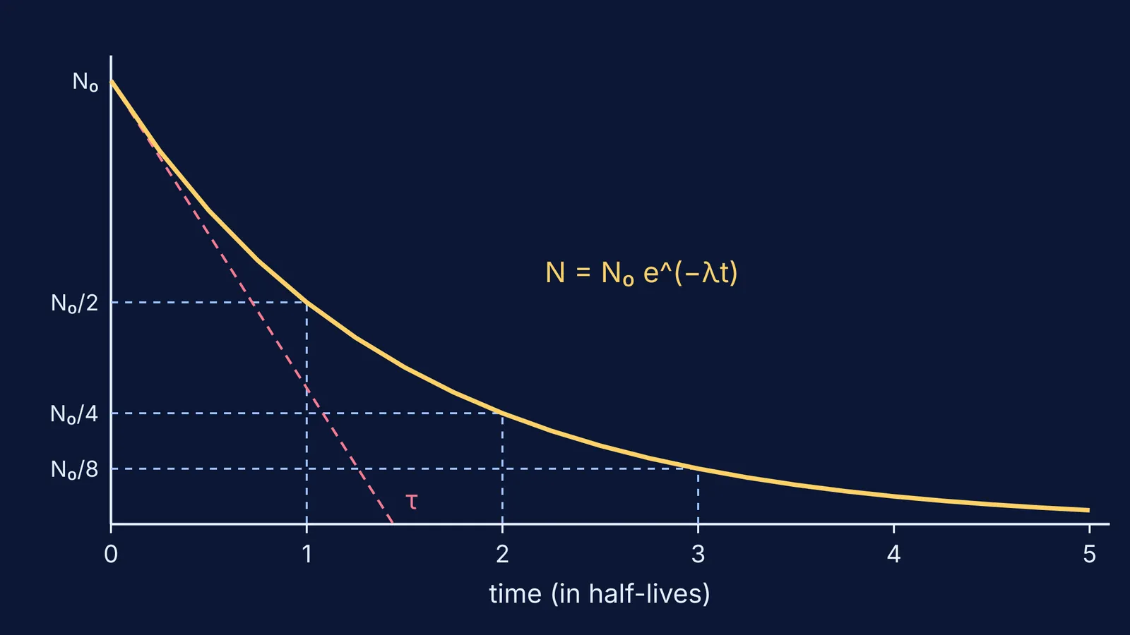
Start from the lottery idea. Give every nucleus the same small chance, λ dt, of decaying in the next short time dt. If you have N nuclei, the expected number that decay is Nλ dt. So the population falls at a rate proportional to how many are left:
dN/dt = −λN
Integrating gives N = N₀ e^(−λt)
Setting N = N₀/2 gives the half-life, T½ = ln 2 / λ ≈ 0.693/λ
HyperPhysics puts it this way: the observed half-life behaviour "can be predicted by assuming that individual nuclear decays are purely random events." The same page notes that the mean lifetime is 1/λ, and the half-life is 0.693 times the mean lifetime.
This is why half-life works. No nucleus remembers its age, so the survivors after one half-life behave like a fresh sample, and the next half-life takes just as long. The smooth law describes the crowd; for one nucleus it gives only a probability. For the exam-side maths, see our guide to radioactive decay and half-life calculations.
How was the randomness of decay tested?
Kohlrausch, Meyer and Regener, and Geiger had already seen the fluctuations by balancing ionisation currents from two sources, with results "in good agreement with the theoretical predictions of von Schweidler" (Rutherford and Geiger, 1910).
Rutherford and Geiger then counted directly. Polonium alpha particles struck a zinc sulphide screen, and each flash was recorded by hand on a moving tape: about 2,000 a day, 10,000 in all, over 5 days. Split into 2,608 intervals of 7.5 seconds, the average was 3.87 particles per interval. The spread matched the formula H. Bateman worked out for them, now called the Poisson distribution: 525 intervals held exactly three particles, against 525 predicted, and 57 held none, against 54 predicted (Rutherford and Geiger, 1910). Read the story of that formula in our post on Siméon Denis Poisson and the maths of rare events.
Worked example: what does random decay mean for your numbers?
Take a made-up nuclide with a half-life of 10 minutes and apply the exponential decay law.
One nucleus. The chance it survives 30 minutes is (1/2)³ = 1/8.
No memory. If it has already survived 20 minutes, the chance it lasts another 10 is still 1/2, not less.
Four nuclei. After one half-life, "two left" is only the most likely outcome. Its probability is 6/16, which is 37.5%. Anything from zero to four can happen.
A counter. Using Schweidler's square-root rule (Rutherford and Geiger, 1910), a count expected to be 100 typically wanders by about 10, which is 10%. A count expected to be 10,000 wanders by about 100, only 1%. Big samples look smooth; small ones look random.
Before a half-life numerical, check two things. Is the sample large enough for the smooth law? Have you measured time from the start of the experiment, not the age of any nucleus?
The jump from random single events to a smooth curve is easier to see than to read, and the Fermi Simulation Lab is built for interactive simulations of ideas like this. If a half-life problem keeps failing at the same step, the Fermi Problem Library has a step-by-step solver that explains the reasoning rather than printing an answer.
The irregular clicks of a Geiger counter are Schweidler's fluctuations made audible: read about Hans Geiger and the counter that made radiation audible.


