

On this page
From heartbeats to seismic rumblings to starlight, physical data often comes to us as waves. To make sense of these complex signals, scientists must break them down into their basic, fundamental frequencies.
The mathematical tool for this job is the Fourier transform. By applying it, a messy time-domain signal reveals the distinct, clean sine waves that make it up. But doing this mathematically on a computer in the early 1960s was incredibly slow, creating a bottleneck in physics, engineering and astronomy.
What made calculating frequencies so slow?
Before 1965, computers calculated the frequencies of a digital signal using the standard Discrete Fourier Transform (DFT). To analyse N data points, the computer had to compare every point against every other point, requiring roughly N² mathematical operations.
For a short 1,024-point audio signal, that brute-force method required over a million multiplications. For a high-resolution signal of a million data points, the computer had to execute a trillion steps. In the early days of computing, when processing power was expensive and scarce, this O(N²) complexity meant that detailed signal analysis was practically impossible.
How did Cooley and Tukey cut the work?
In April 1965, James W. Cooley of IBM and John W. Tukey of Princeton University published "An algorithm for the machine calculation of complex Fourier series" in the journal *Mathematics of Computation*. They introduced a "divide and conquer" approach to the Fourier transform.
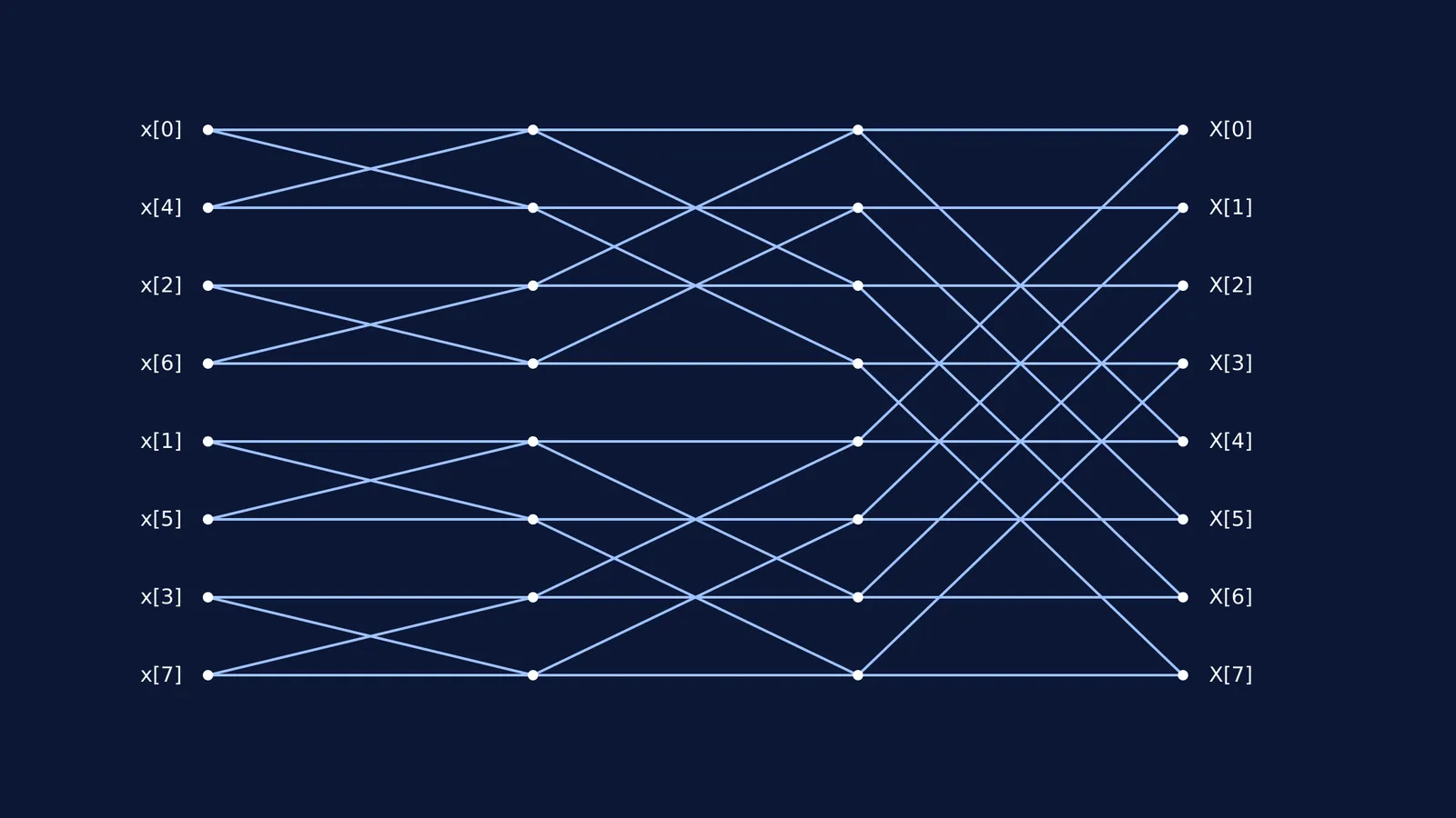
Instead of tackling all N data points at once, their algorithm split the problem into two halves: the even-numbered data points and the odd-numbered ones. It then split those halves into quarters, the quarters into eighths, and so on, right down to pairs of points. By solving the smallest problems first and combining the results—using a structure now known as a butterfly diagram—they reused calculations and bypassed the redundant work of the standard DFT.
According to the mathematical principles of the Cooley-Tukey algorithm, this recursive splitting reduced the required operations from O(N²) to exactly O(N log₂ N). For a 1,024-point wave, the number of operations plummeted from 1,048,576 to just 10,240. What previously took a computer hours could now be done in fractions of a second.
If you are stuck on the mathematics of waves or the trigonometric identities behind these calculations, Fermi's AI tutor can work out what you already know and build a plan for the session, so you sit down to a clear next step.
Why does the 1965 Fast Fourier Transform matter today?
The Fast Fourier Transform (FFT) became an immediate sensation. It was initially developed in part to help the US military analyse seismic waves to differentiate natural earthquakes from underground nuclear tests during the Cold War.
Today, the FFT is the invisible backbone of modern digital life. When your smartphone connects to a Wi-Fi router, it uses the FFT to quickly decode the incoming electromagnetic waves. When you compress a photograph into a JPEG or listen to an MP3, a variant of the FFT isolates the most important visual or audio frequencies so the rest can be discarded to save space. In hospitals, MRI machines rely on the FFT to reconstruct detailed images of the human body from raw magnetic resonance data.
If you are having trouble picturing how a single complex wave decomposes into distinct frequency components, the Fermi Simulation Lab provides interactive simulations for ideas that are easier to see than read.
How do you spot an O(N log N) divide-and-conquer problem?
The brilliance of the 1965 FFT paper was recognising that the Fourier transform was packed with redundant calculations that could be factored out by dividing the dataset. If you are studying computer science or advanced mathematics, you can spot opportunities to speed up an O(N²) algorithm to O(N log N) by looking for these three signs:
Divisibility: Can the main problem be cleanly split into two or more smaller, identical versions of itself? (In the FFT, a large Fourier transform splits into two smaller transforms).
Independence: Do the smaller sub-problems avoid interfering with each other?
Cheap combination: Can you merge the answers of the smaller problems back together with very little computational effort?
When an algorithm meets these criteria, applying a recursive, divide-and-conquer strategy will almost always result in a massive reduction in processing time. Just as understanding displacement and pressure waves is essential to acoustics, mastering this mathematical framework is foundational to modern computer science.


