

On this page
In 665 CE, the Indian mathematician and astronomer Brahmagupta completed the *Khandakhadyaka*, a major text on astronomy and mathematics. To track planetary positions, astronomers needed precise values of the sine function (the half-chord or *jya*) for angles not listed in their standard tables. While earlier mathematicians like Aryabhata used simple linear interpolation, Brahmagupta introduced a more accurate method using second-order differences.
What is Brahmagupta's second-order interpolation formula?
When a function's values are known at equal intervals, interpolation finds the value at a point in between. Brahmagupta's formula was a second-order polynomial interpolation, mathematically equivalent to the modern Newton-Stirling interpolation formula truncated at the second-order differences.
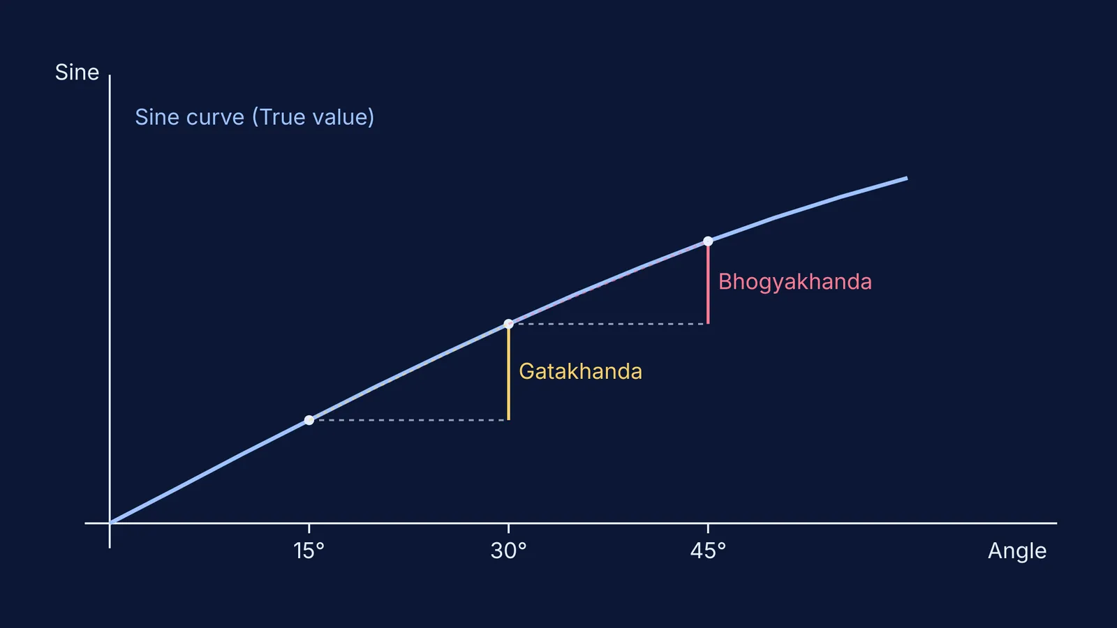
He defined the interval between tabulated points as h (which in his tables was 900 minutes, or 15 degrees). To find the value at a fractional distance along this interval, his rule combined two key differences. The first was the *gatakhanda*, which is the difference between the current tabular value and the previous one. The second was the *bhogyakhanda*, the difference between the next tabular value and the current one.
How did the Khandakhadyaka compute sine values?
In the *Khandakhadyaka*, Brahmagupta described the mathematical steps in a Sanskrit couplet. He instructed astronomers to multiply the remaining angle in minutes (the *vikala*) by half the difference of the *gatakhanda* and *bhogyakhanda*, and then divide by 900.
This result was then added to or subtracted from the mean of the two differences to yield the "corrected" tabular difference, which he called the *sphuta-bhogyakhanda*. This correction meant his sine table calculations accounted for the curve of the sine wave, reducing the errors that arise when assuming the function is a straight line between points.
Why is second-order interpolation important for students today?
Recognising patterns in differences is a core skill in sequences, series, and numerical methods problems. The step from linear to second-order interpolation marks the historical transition from arithmetic approximation to early calculus-style thinking. For instance, when you learn to derive the exact values of sin 18° and cos 36° or use sin 3x, cos 3x and tan 3x formulas in trigonometry, you are building on the same historical pursuit of precise angles.
If you are solving numerical methods or sequence problems and get stuck on finding the pattern of differences, the Fermi Problem Library provides worked problems with a step-by-step solver that explains the reasoning rather than just printing an answer. When you need to brush up on the underlying trigonometric identities, the Fermi Concept Library holds a lesson for every concept in physics, chemistry, biology, mathematics and computing, each with its place in the map.


