On this page
The discovery that electricity creates magnetism sparked a race among physicists. In 1820, Jean-Baptiste Biot and Félix Savart turned a surprising observation into a precise mathematical formula, giving us the Biot-Savart law.
In the summer of 1820, Danish physicist Hans Christian Ørsted noticed that an electric current could deflect a nearby compass needle. When this news reached Paris, scientists rushed to understand the effect. While André-Marie Ampère began building a broad theoretical framework, Biot and Savart focused on finding the exact mathematical relationship through precise measurements.
Today, their law is a cornerstone of electromagnetism. It explains everything from the forces in electric motors to the paths of charged particles in accelerators, and remains a core topic for physics students preparing for exams like the JEE and NEET.
How did Biot and Savart measure the magnetic field?
Without modern digital magnetometers, Biot and Savart had to rely on classical mechanics to measure an invisible field. They placed a small, magnetized compass needle near a long, vertical wire carrying a steady current from an early battery.
Why does the period of oscillation measure the magnetic field?
Biot and Savart used the method of oscillations to measure the field's strength. When the magnetic needle is slightly pushed, the magnetic field acts as a restoring force, making the needle swing back and forth.
Just as a pendulum swings faster in a stronger gravitational field, the magnetic needle oscillates faster in a stronger magnetic field. The physics dictate that the magnetic field strength (B) is inversely proportional to the square of the oscillation period (B ∝ 1/T²). By carefully timing these swings at various distances (r) from the wire, they gathered their data.
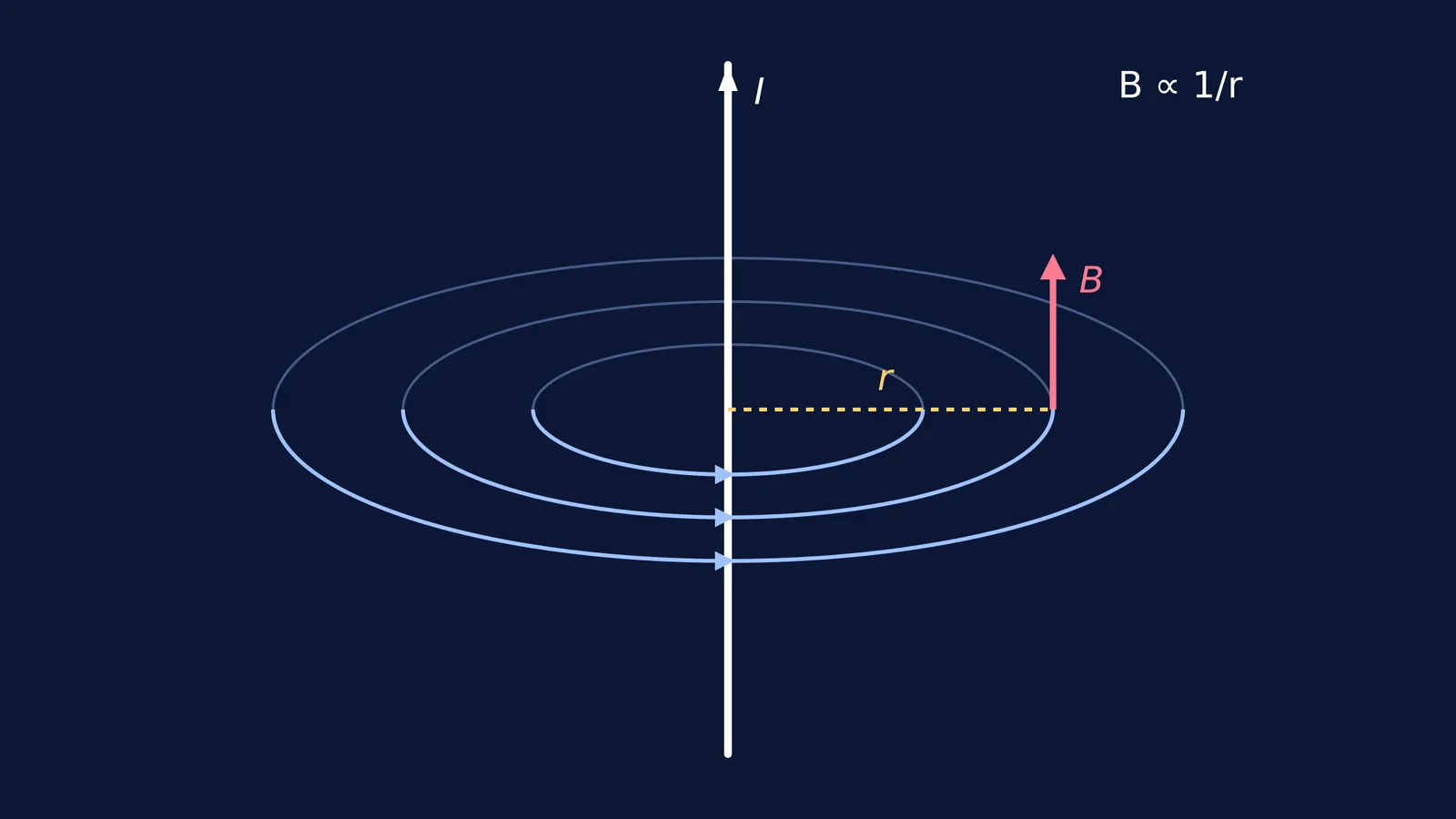
Their results showed a clear pattern: when the distance from the wire doubled, the period squared quadrupled, meaning the magnetic force was halved, as detailed in the history of the Biot-Savart law. They concluded that the magnetic field of an infinitely long straight wire is inversely proportional to the distance from it (B ∝ 1/r).
If you find yourself stuck trying to set up the calculus for these infinitesimal slices, Fermi's AI tutor can help. It doesn't just print the final integral; it holds a line of reasoning, draws the figure, and helps you work out the geometry step by step.
How to calculate the magnetic field of a straight wire?
From Biot and Savart's 1820 measurement, we get the modern formula for the magnetic field magnitude at a distance r from a long, straight wire carrying current I:
B = μ₀ I / 2πr
Here, μ₀ is the permeability of free space. The direction of this field is found using the right-hand rule: if you point your right thumb in the direction of the current, your fingers curl in the direction of the circular magnetic field lines.
Visualising these invisible 3D vector fields is often the hardest part of learning electromagnetism. If static textbook diagrams leave you confused about which way the vectors point, the Fermi Simulation Lab lets you interact with 3D models of currents and fields to see them clearly.
Once you master the straight wire, you can apply the same principles to more complex problems, such as finding the circulating electric field inside a changing solenoid or predicting the helical path of a charge moving through a magnetic field.