

On this page
When you learn linear programming—whether for your Class 12 board exams or when finding area using horizontal strips—you spend a lot of time shading graphs. You draw lines for your constraints, find the overlapping shape (the feasible region), and then test only the corner points to find the maximum or minimum value.
But why do we skip the millions of points in the middle? The answer lies in the geometry of linear equations and a mathematical rule known as the fundamental theorem of linear programming.
The geometry of a straight line
Every linear programming problem (LPP) has an objective function, usually written as Z = ax + by. This is the value you want to maximise (like profit from selling two different products) or minimise (like the cost of two types of raw materials).
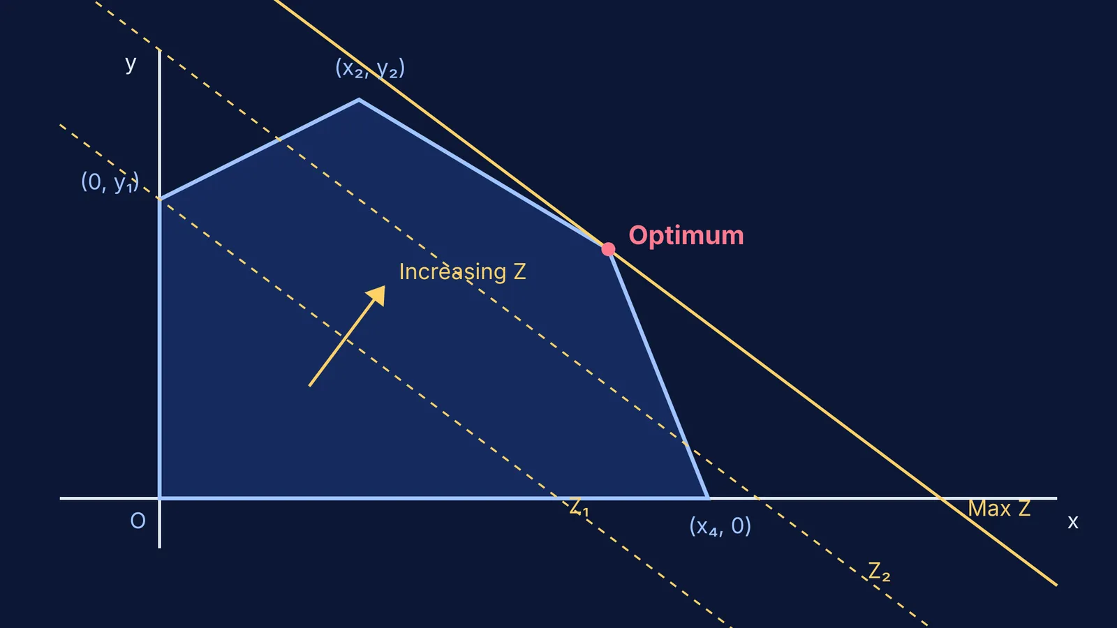
Because the equation is strictly linear, it has no curves, peaks, or valleys. If you pick a specific value for Z, the equation ax + by = Z forms a straight line on your graph. If you increase Z (while keeping a and b constant), that line moves in a parallel direction across the coordinate plane. The slope of this line depends purely on the ratio of a and b, which means the line keeps its exact angle as it sweeps across the graph.
The feasible region—the area bounded by your constraints—forms a convex polygon. A shape is convex if you can draw a straight line between any two points inside it without crossing outside the boundary.
If you imagine the objective function as a sliding parallel line moving in the direction of improvement, it will sweep across this flat, convex polygon. Because the boundary is made of straight segments meeting at angles, the "last point" the line touches before leaving the region completely will always be a vertex, or corner. Moving any further in that direction would take you outside the allowed region, violating one of your constraints. Stopping earlier in the middle of the shape would mean there is still room to improve the value further.
Why does the optimum occur at a corner point?
This geometric reality gives us the corner point theorem: if a linear programming problem has a bounded optimal solution, it must occur at a corner point of the feasible region. You never have to test the infinite points in the interior.
This idea is the basis for the Simplex algorithm, a mathematical method developed by George Dantzig in 1947 1. Rather than graphing lines on paper, Dantzig's algorithm navigates the edges of multi-dimensional shapes to find optimal solutions efficiently, forming the backbone of modern logistics and operations research.
What if two corner points give the same result?
Sometimes, when you test your corner points, you find that two adjacent vertices give the exact same maximum or minimum value.
This happens when the sliding objective function line is perfectly parallel to one of the polygon's edges. Instead of leaving the shape at a single vertex point, the line sits flush against the entire boundary edge. In this case, not only are the two corner points optimal, but every single point on the line segment connecting them is also an optimal solution. This means the problem has infinitely many valid solutions that all give the exact same optimal value for Z.
How do you use the corner point method?
Setting up constraints and finding intersection points can be error-prone. The Fermi Problem Library has worked problems with a step-by-step solver that explains the reasoning rather than printing an answer.
When you tackle a linear programming problem on paper, follow this sequence to ensure you catch the correct optimum every time:
Graph the constraints: Draw each linear inequality as a boundary line and shade the allowed side. Use a sharp pencil and a ruler; small sketching errors can lead you to the wrong corners.
Find the feasible region: Identify the convex polygon where all shaded areas overlap. Remember to include the non-negativity constraints (x ≥ 0, y ≥ 0), which restrict your shape to the first quadrant.
Locate the vertices: Find the exact coordinates of every corner point. You cannot always read these from a graph; you may need to solve simultaneous equations for lines that cross, much like when counting intersections of two sketched curves.
Test the function: Substitute the (x, y) coordinates of each corner into your objective function Z. Create a clear table with a row for each corner point to avoid calculation mistakes.
Pick the optimum: The highest value is your maximum, and the lowest is your minimum. If your region is unbounded, run the open half-plane test to verify the solution.
Understanding why this graphical method works means you never have to second-guess whether a better answer is hiding in the middle of your graph. Because the objective function is a straight line sweeping across a convex shape, the optimum is always waiting at the very edge.
Try your next linear programming question in the Fermi Problem Library.


