

On this page
A differential equation is an equation that relates an unknown function to its own derivatives. While finding a solution from scratch can be difficult, verifying that a given function is a solution is much simpler. It comes down to basic differentiation and algebra, much like proving relations with second-order derivatives.
How to verify that a function is a solution of a differential equation?
Verifying a solution is essentially a "plug-and-check" process. You must prove that when you substitute the proposed function and its derivatives into the equation, the left side exactly equals the right side for all values in the domain.
Here is the step-by-step method:
Find the derivatives: Look at the differential equation to see the highest derivative it requires. Differentiate your proposed function up to that order.
Substitute: Replace every instance of the function and its derivatives in the differential equation with the expressions you just calculated.
Simplify: Expand and combine like terms.
Compare: If both sides simplify to an identical match (such as 0 = 0), the function is a verified solution.
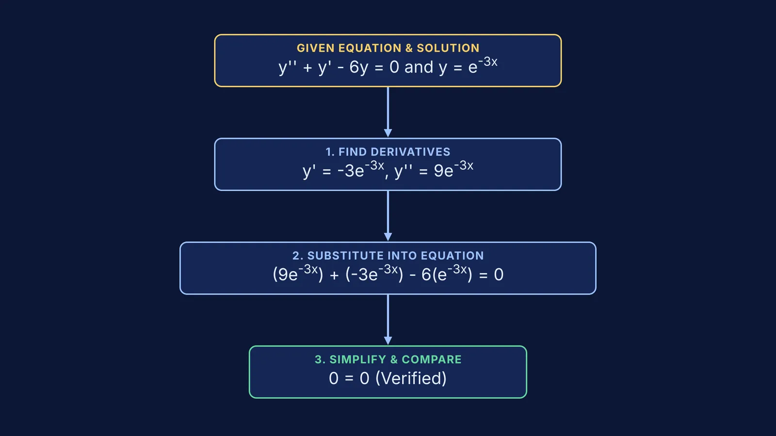
For example, let's verify that y = e^(-3x) is a solution to the second-order equation y'' + y' - 6y = 0.
First, we find the derivatives:
y' = -3e^(-3x)
y'' = 9e^(-3x)
Next, we substitute these into the equation: (9e^(-3x)) + (-3e^(-3x)) - 6(e^(-3x)) = 0
Finally, we simplify by factoring out e^(-3x): (9 - 3 - 6)e^(-3x) = 0 0 = 0
Since the equation holds true, the function is a verified solution. If you drop a sign or make an algebra mistake during substitution, the sides will not match. When that happens, the Fermi Problem Library has worked problems with a step-by-step solver that explains the reasoning rather than printing an answer, helping you spot where the substitution went wrong.
Why does the number of arbitrary constants equal the order?
When you solve a differential equation, you are essentially working backwards from a derivative to the original function. The highest derivative in the equation is called its order.
According to Math LibreTexts/08%3A_Introduction_to_Differential_Equations/8.01%3A_Basics_of_Differential_Equations), the number of arbitrary constants in a general solution is exactly equal to the order of the differential equation.
This happens because undoing a derivative requires integration. Every time you integrate an expression, you introduce one arbitrary constant of integration (usually written as C).
To solve a first-order equation (which only has y'), you integrate once, yielding one constant (C).
To solve a second-order equation (which has y''), you must integrate twice, yielding two independent constants (C₁ and C₂).
A general solution contains all of these arbitrary constants, representing an entire family of curves that satisfy the equation.
What is the difference between a general and particular solution?
A general solution includes the arbitrary constants and covers all possible answers. For example, the general solution to the first-order equation y' = 2x is y = x² + C. (You will often see these constants when solving growth and cooling exponential models).
A particular solution is a single, specific function where the constants have been replaced with real numbers, such as y = x² + 4. You find these specific numbers by using initial conditions provided in the problem.
How do you verify an initial value problem?
An initial value problem (IVP) is a differential equation paired with specific starting conditions, such as y(0) = 3. As noted by Math LibreTexts/08%3A_Introduction_to_Differential_Equations/8.01%3A_Basics_of_Differential_Equations), the number of initial values needed to solve an IVP is typically equal to the order of the differential equation, allowing you to find a value for every arbitrary constant.
To verify a solution to an IVP, you must pass two tests:
Verify the equation: Differentiate and substitute the function to ensure it satisfies the differential equation, just as you would for a general solution.
Verify the initial condition: Substitute the given x-value into the proposed function and check if it produces the required y-value.
For example, to verify that y = 2e^(-2t) + e^t is a solution to the IVP y' - y = -6e^(-2t) with the condition y(0) = 3, you first plug the function into the equation. Once that checks out, you plug t = 0 into the function: y(0) = 2e^0 + e^0 = 2(1) + 1 = 3.
Since the result matches the initial condition, the particular solution is fully verified.


