

On this page
In Class 11 physics, standard problems in JEE Main and NEET-UG provide a particle's position as a cubic polynomial in time, such as x(t) = t³ − 6t² + 9t, and ask for the total distance traveled or the acceleration when the particle stops. Solving these problems requires three steps: differentiating position to find velocity, setting velocity to zero to identify turning points, and splitting the time interval at those turning points to sum the true path length.
How do you find when velocity is zero from x(t)?
Instantaneous velocity is the time derivative of position, v(t) = dx/dt. When position is given by a cubic equation x(t) = At³ + Bt² + Ct + D, differentiating yields a quadratic velocity function: v(t) = 3At² + 2Bt + C.
To find when the particle comes to rest, set v(t) = 0 and solve 3At² + 2Bt + C = 0 for time t. The real, non-negative roots mark the instants when velocity vanishes.
In a study of 895 students published in the American Journal of Physics, Robert J. Beichner documented that learners often suffer from slope and height confusion, mistakenly reading a coordinate value when asked for a rate of change. Earlier work by David E. Trowbridge and Lillian C. McDermott in the American Journal of Physics showed that students often rely on a "position criterion", assuming an object at x = 0 is stopped or that passing another object implies equal velocity.
Recognizing that zero velocity means a horizontal tangent on an x-t graph clears up this confusion. Fermi's AI tutor notices where a student is stuck and holds a line of reasoning across a session to clarify how derivatives describe motion before moving to algebraic steps.
Why is distance different from displacement at turning points?
The most common trap in calculus kinematics is equating distance with displacement. Displacement is the vector change in position, ∆x = x(t_final) − x(t_initial). Forward motion (v > 0) and backward motion (v < 0) cancel each other out in the net displacement. Distance is the scalar total path length, which never decreases.
Whenever a particle reverses direction, velocity changes sign. If you evaluate x(t_final) − x(t_initial) across an interval containing a reversal, the return trip cancels part of the forward journey. To find true distance, you must locate every turning point where v = 0 within the window, confirm that velocity changes sign, and sum the absolute displacements of each segment.
This distinction is central when distinguishing average speed from average velocity, where speed depends on path length and velocity depends on displacement.
What is the step-by-step method for cubic position problems?
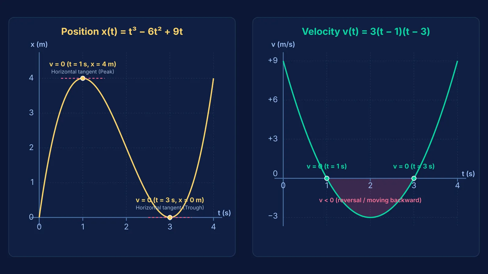
Consider a standard problem: a particle moves along the x-axis with position x(t) = t³ − 6t² + 9t (in metres and seconds). Find when velocity is zero, the acceleration at those times, and the total distance traveled from t = 0 to t = 4 s.
Differentiate position to find velocity: v(t) = dx/dt = 3t² − 12t + 9 = 3(t − 1)(t − 3).
Set velocity to zero: 3(t − 1)(t − 3) = 0 gives t = 1 s and t = 3 s. Both roots lie inside [0, 4 s].
Differentiate velocity to find acceleration: a(t) = dv/dt = 6t − 12. At t = 1 s, a(1) = −6 m/s². At t = 3 s, a(3) = +6 m/s². Even when velocity is zero, acceleration can be non-zero. In the American Journal of Physics, Trowbridge and McDermott showed that students often struggle to separate velocity from acceleration, wrongly assuming that zero velocity requires zero acceleration.
Evaluate positions at key times: x(0) = 0 m, x(1) = 4 m, x(3) = 0 m, and x(4) = 4 m.
Sum absolute displacements between consecutive critical times:
Segment 1 (t = 0 to 1 s): |x(1) − x(0)| = |4 − 0| = 4 m.
Segment 2 (t = 1 to 3 s): |x(3) − x(1)| = |0 − 4| = 4 m.
Segment 3 (t = 3 to 4 s): |x(4) − x(3)| = |4 − 0| = 4 m.
Total distance = 4 + 4 + 4 = 12 m.
Displacement over four seconds is only x(4) − x(0) = 4 m. Relying on displacement misses two-thirds of the total motion. This method connects directly to calculus maxima and minima and techniques for integrating variable acceleration.
When tackling multi-step mechanics questions, the Fermi Problem Library provides worked problems with a step-by-step solver that explains the reasoning rather than printing an answer. To review underlying kinematics principles, the Fermi Concept Library covers every concept in physics, chemistry, biology, mathematics and computing, each with its own lesson and its place in the map.


