

On this page
In probability theory, the mathematical foundation rests on a set of rules called the Kolmogorov axioms. When you first encounter the axiomatic approach to probability in Class 11 mathematics, you are often asked to look at a list of numbers and check whether the assignment of probabilities is valid.
The idea is simple: you have a random experiment with a sample space S = {w₁, w₂, ..., wₙ}, which is the set of all possible outcomes. Before you can calculate the probability of any larger event, you must assign a probability P(wᵢ) to each individual outcome. But you cannot pick just any numbers.
The axiomatic approach to probability
In 1933, the mathematician Andrey Kolmogorov introduced a formal mathematical foundation for probability. His axioms define a probability space through core rules: probabilities must be non-negative, the total probability of the entire sample space must equal one, and the probability of mutually exclusive events is the sum of their individual probabilities.
This axiomatic approach removed the ambiguity from classical probability, which relied on the assumption that all outcomes are equally likely. In the real world, a biased coin or a loaded die does not have equally likely outcomes. The axiomatic approach allows us to handle these situations, provided the numerical assignment of probabilities remains valid.
What makes an assignment of probabilities valid?
For a probability assignment to be mathematically correct, it must satisfy two fundamental conditions.
Non-negativity: The probability of each individual outcome must be between 0 and 1, inclusive. Mathematically, 0 ≤ P(wᵢ) ≤ 1 for each outcome i. No probability can be negative, and no single outcome can have a probability greater than 1.
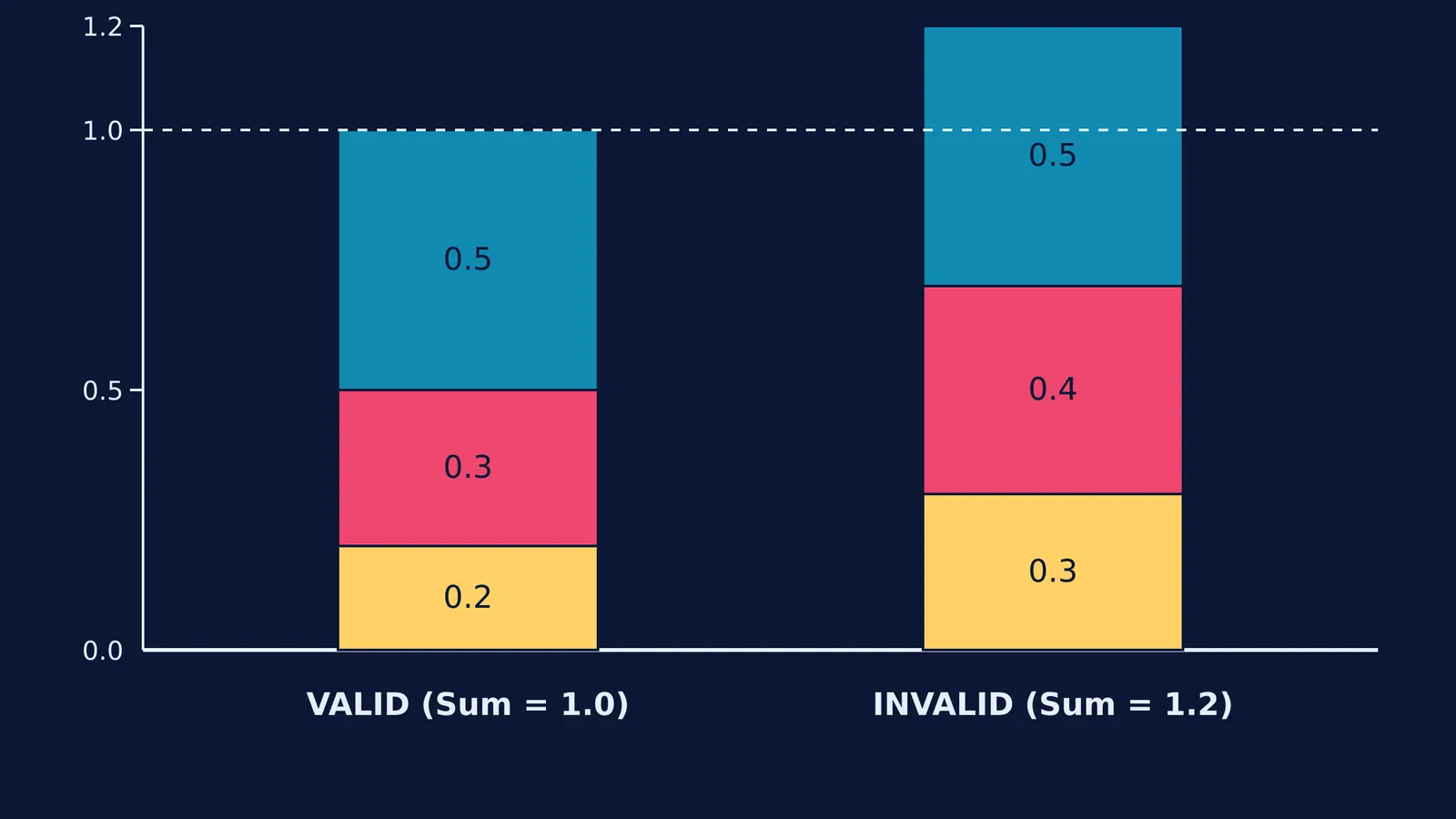
Sum of probabilities: The sum of the probabilities of all possible outcomes in the sample space must be exactly 1. In symbols, P(w₁) + P(w₂) + ... + P(wₙ) = 1. This means that some outcome in the sample space is guaranteed to happen.
If an assignment fails even one of these conditions, it is invalid.
How to check whether assignment of probabilities is valid?
When you face a test question with a list of assigned probabilities for outcomes w₁ through w₅, use this simple checklist:
Scan for negatives: Are there any negative numbers? If yes, reject the assignment immediately.
Scan for numbers greater than 1: Are there any values like 1.2 or 3/2? If yes, reject it.
Add them up: Sum all the values. If the total is 0.99 or 1.05, the assignment is invalid. It must be exactly 1.
Let us look at some examples for a sample space with five outcomes.
Example A: 0.2, 0.2, 0.2, 0.2, 0.2
Are they all between 0 and 1? Yes.
Do they sum to 1? 0.2 + 0.2 + 0.2 + 0.2 + 0.2 = 1.0.
Verdict: Valid.
Example B: -0.1, 0.3, 0.4, 0.2, 0.2
Are they all between 0 and 1? No, the first value is -0.1.
Verdict: Invalid. You do not even need to check the sum.
Example C: 0.1, 0.2, 0.3, 0.4, 0.5
Are they all between 0 and 1? Yes.
Do they sum to 1? 0.1 + 0.2 + 0.3 + 0.4 + 0.5 = 1.5.
Verdict: Invalid. The total exceeds 1.
Sometimes, checking these rules involves dealing with messy fractions or algebra, and not knowing where to start can stall your practice. The Fermi Concept Library explains every concept in physics, chemistry, biology, mathematics and computing. If you get stuck on an assignment of probabilities, Fermi's AI tutor can work out what you already know and build a plan for the session, guiding you through the conditions one by one.
What if all outcomes are equally likely?
In many familiar experiments, such as rolling a fair die or tossing a coin, every outcome has the same chance of occurring. If a sample space has n equally likely outcomes, the probability assigned to each outcome is exactly 1/n.
For example, a fair die has six outcomes: S = {1, 2, 3, 4, 5, 6}. Because they are equally likely, each outcome is assigned a probability of 1/6. Since all six values are between 0 and 1, and their sum (6 × 1/6) equals 1, this is a valid assignment.
How to find the probability of an event?
Once you have verified that the assignment of probabilities is valid, you can calculate the probability of any event. An event is simply a subset of the sample space. To find its probability, you add the probabilities of the individual outcomes that make up that event.
For example, suppose you have a valid assignment for a biased six-sided die where P(1) = 0.1, P(2) = 0.1, P(3) = 0.1, P(4) = 0.1, P(5) = 0.2, and P(6) = 0.4.
If event A is "rolling an even number", then A = {2, 4, 6}. The probability of event A is: P(A) = P(2) + P(4) + P(6) = 0.1 + 0.1 + 0.4 = 0.6.
This straightforward addition is why the rule that the total must be exactly 1 is so important. If the total probability of the sample space were greater than 1, you could end up calculating a probability greater than 1 for a certain event, which is mathematically meaningless.
Mastering this fundamental check prepares you for more advanced topics. Whether you are dealing with with and without replacement probability problems or solving three-set Venn problems using inclusion-exclusion, every calculation relies on a valid initial assignment.


