

On this page
When preparing for school or competitive exams like JEE Main, students often sketch quadratics by compiling an arbitrary table of values and connecting the dots. This point-plotting habit frequently produces distorted, lopsided, or V-shaped graphs. In a foundational review in *Review of Educational Research*, Leinhardt, Zaslavsky, and Stein (1990) showed that students struggle because they rely on local point-by-point calculation rather than interpreting global features like symmetry and extrema. Furthermore, in an exploratory study of 178 secondary mathematics students, Knuth (2000) found that learners overwhelmingly default to algebraic manipulation without connecting equations to their underlying Cartesian graphs.
To sketch a parabola accurately and quickly, you do not need an exhaustive table of values. You only need five key landmarks plotted in order: opening direction, vertex, axis of symmetry, y-intercept, and x-intercepts, confirmed by one quick check point.
What are the key features needed to sketch a parabola?
Every quadratic function can be expressed in standard form as y = ax² + bx + c, where a ≠ 0. Its graph depends directly on these coefficients:
Opening direction: If a > 0, the parabola opens upward, holding a minimum at its base. If a < 0, it opens downward, holding a maximum at its peak.
Vertex: The turning point where x_v = −b/(2a). Substituting x_v yields y_v = −D/(4a), where D = b² − 4ac is the discriminant.
Axis of symmetry: The vertical line x = −b/(2a) that bisects the curve into two mirror-image arms.
y-intercept: Setting x = 0 gives (0, c), the point where the curve crosses the vertical axis.
x-intercepts: Setting y = 0 gives ax² + bx + c = 0. The discriminant D determines the roots: two distinct intercepts if D > 0, one touching vertex if D = 0, and no real intercepts if D < 0.
How do you sketch a parabola step by step?
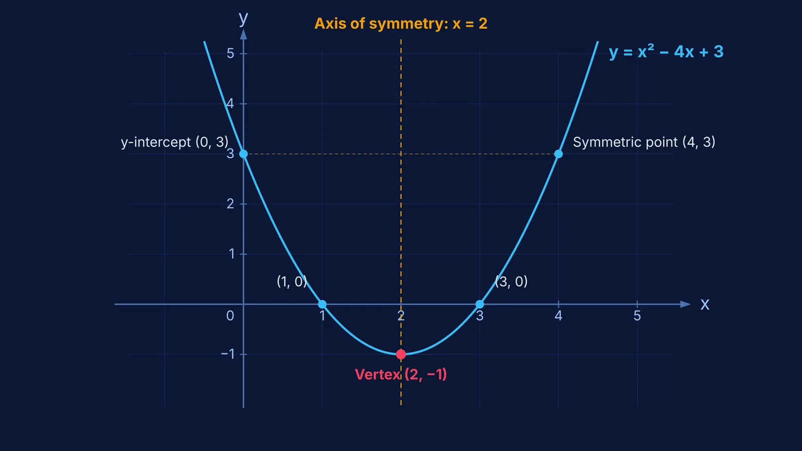
To see how these landmarks guide your pencil, sketch y = x² − 4x + 3:
Opening direction: Here a = 1 > 0, so the parabola opens upward.
Vertex: Calculate x_v = −(−4)/(2 × 1) = 2. Then y_v = (2)² − 4(2) + 3 = −1. Plot the vertex at (2, −1).
Axis of symmetry: Draw a vertical dashed line down x = 2 as your balance guide.
y-intercept and reflection: Set x = 0 to get (0, 3). Because (0, 3) lies at a distance of 2 to the left of the axis x = 2, reflect it across the axis to plot its twin at (4, 3).
x-intercepts: Set y = 0. Factoring x² − 4x + 3 = 0 gives (x − 1)(x − 3) = 0, yielding x = 1 and x = 3. Plot (1, 0) and (3, 0), which sit symmetrically at distance 1 on either side of x = 2.
Quick check point: Test x = 5: y = 5² − 4(5) + 3 = 8. Plot (5, 8) to confirm your curve rises smoothly.
Draw a rounded U-shape through the vertex at (2, −1), rising through (1, 0) and (3, 0), and extending past (0, 3) and (4, 3).
When working through multi-step graphing problems, the Fermi Problem Library has worked problems with a step-by-step solver that explains the reasoning rather than printing an answer.
What if the quadratic equation has no real x-intercepts?
When a quadratic has a negative discriminant (D < 0), ax² + bx + c = 0 yields complex roots, leading many students to assume the graph cannot be drawn. In reality, D < 0 simply means the curve never crosses the x-axis. If a > 0, the parabola floats entirely above the horizontal axis; if a < 0, it sinks entirely beneath it.
Consider y = x² − 2x + 3, where D = (−2)² − 4(1)(3) = −8 < 0. Because D < 0 and a > 0, there are no real x-intercepts. You still sketch it effortlessly:
Vertex: x = −(−2)/2 = 1, giving y = (1)² − 2(1) + 3 = 2. Plot (1, 2).
Axis: x = 1.
y-intercept: (0, 3). Reflect across x = 1 to plot (2, 3).
Check point: at x = 3, y = 6; by symmetry, x = −1 also gives y = 6.
Understanding this geometry is crucial for solving inequalities, as explained in When is ax² + bx + c positive for all x? The discriminant test. It also underpins questions on root placement, examined in Quadratic equations for JEE: nature and location of roots. In calculus, accurate sketches ensure correct integration limits, as shown in Area under curves: sketch first, then integrate.
To build intuition across algebra and geometry, the Fermi Concept Library covers every concept in physics, chemistry, biology, mathematics and computing, each with its own lesson and its place in the map. As you practice, Fermi's AI tutor can work out what you already know and build a plan for the session, drawing figures on a board and checking understanding as you work through each graph.


