How to recognise a second-order reaction from a 1/[A] plot

When you track how fast a chemical reaction runs, the changing concentration of the reactants tells you the reaction's order. For a second-order reaction involving a single reactant, plotting the reciprocal of concentration against time is the definitive test.

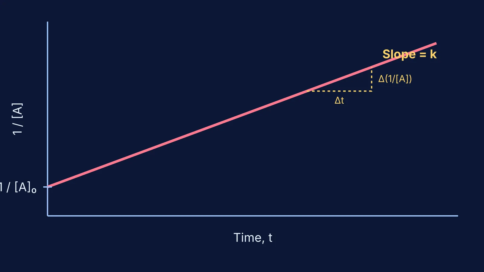
According to OpenStax Chemistry 2e, a plot of 1/[A] versus time for a second-order reaction yields a straight line where the slope is the rate constant, k. If you plot the same data as simply [A] against time or ln[A] against time, you will get a curve instead.

How to recognise a second-order reaction from a 1/[A] plot?

A reaction is second-order with respect to a reactant A if its rate is proportional to the square of that reactant's concentration. The rate law is written as Rate = k[A]².

When you integrate this differential rate equation, you get the integrated rate law for a second-order reaction: 1/[A] = kt + 1/[A]₀

This is the equation of a straight line (y = mx + c).

• The y-axis is 1/[A], the reciprocal of the concentration at time t.

• The x-axis is time, t.

• The slope is the rate constant, k. Because k is positive, the line slopes upwards.

• The y-intercept is 1/[A]₀, which is the reciprocal of the initial concentration.

If you are given experimental data and asked to find the order, you can test it by graphing. Just as integrated rate law graphs show a straight line for ln[A] in a first-order process, only a second-order process will give a straight line for 1/[A].

How does this compare to zero and first-order reactions?

To be certain a reaction is second-order, you often need to rule out zero-order and first-order possibilities.

• For a zero-order reaction, the rate is independent of concentration. A plot of simply [A] against time yields a straight line with a negative slope. If you plot 1/[A] for a zero-order reaction, you get a curve that bends upwards.

• For a first-order reaction, the rate is proportional to the concentration. A plot of the natural logarithm, ln[A], against time yields a straight line with a negative slope. If you plot 1/[A] for a first-order reaction, you also get a curve.

Only when the reaction is second-order with respect to a single reactant will the plot of 1/[A] versus time be perfectly straight. Because the slope is positive k, the line will rise from left to right, whereas the straight-line plots for zero and first-order reactions fall.

Why does the half-life increase over time?

The half-life (t₁/₂) is the time it takes for half of the reactant to be consumed. For a second-order reaction, the OpenStax Chemistry 2e textbook gives the formula as t₁/₂ = 1 / (k[A]₀).

This means the half-life is inversely proportional to the initial concentration.

• In a first-order reaction, the half-life is constant.

• In a second-order reaction, as the reactant is used up and the concentration falls, the half-life grows longer.

For example, if the first half-life takes 10 seconds, the concentration has halved. For the next interval, the "initial" concentration is now half of what it was, which means the next half-life will take 20 seconds. The third will take 40 seconds.

If you struggle with the calculus needed to integrate rate laws, the Fermi Concept Library holds every concept in physics, chemistry, biology, mathematics and computing, each with its own lesson and its place in the map. It shows you exactly how the differential equation becomes a straight-line graph.

How can you check data without drawing a graph?

You do not always need to draw a graph to check for a straight line. You can test the data by calculating 1/[A] and checking if it increases by a constant amount in equal time steps, a method demonstrated in OpenStax Chemistry 2e.

Consider this hypothetical data for a decomposition reaction:

1. At 0 seconds, [A] is 0.500 mol/L.

2. At 10 seconds, [A] is 0.333 mol/L.

3. At 20 seconds, [A] is 0.250 mol/L.

4. At 30 seconds, [A] is 0.200 mol/L.

Let us find the reciprocal, 1/[A], for each point:

• At 0 seconds, 1/0.500 = 2.0 L/mol

• At 10 seconds, 1/0.333 ≈ 3.0 L/mol

• At 20 seconds, 1/0.250 = 4.0 L/mol

• At 30 seconds, 1/0.200 = 5.0 L/mol

For every 10-second step, the value of 1/[A] increases by exactly 1.0 L/mol. Because the rate of change of 1/[A] is constant, a plot of these points would form a perfect straight line, proving the reaction is second-order.

We can also read the rate constant directly from these numbers. The slope k is the change in 1/[A] divided by the change in time. Using the first 10 seconds: k = (3.0 − 2.0) / 10 = 0.10 L mol⁻¹ s⁻¹.

(Remember that this only holds at a constant temperature, because the temperature coefficient of reaction rate dictates that k shifts when the temperature changes.)

When you know the rate constant, you can predict how much reactant remains at any future time. If you get stuck applying the formula to homework questions, the Fermi Problem Library has worked problems with a step-by-step solver that explains the reasoning rather than printing an answer.