

On this page
Calculating the determinant of a 3×3 matrix using standard cofactor expansion can be tedious. You have to extract three smaller 2×2 matrices, multiply them by the top-row elements, and remember to alternate the signs. One dropped negative sign ruins the entire calculation.
In the 19th century, French mathematician Pierre Frédéric Sarrus (1798–1861) published a visual shortcut that bypasses the nested brackets entirely. By arranging the numbers in a wider grid, you can find the determinant using only straight diagonal lines.
What is Sarrus' rule?
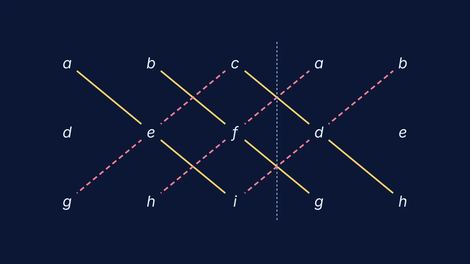
To use Sarrus' rule on a 3×3 matrix, you first write down the matrix. Then, take the first two columns and copy them exactly to the right of the matrix. This gives you a grid that is three rows tall and five columns wide.
Now, draw three diagonal lines starting from the top-left, going downwards and to the right. Each line will pass through exactly three numbers. Multiply the three numbers on each line, and add these three products together.
Next, draw three diagonal lines starting from the bottom-left, going upwards and to the right. Again, multiply the three numbers on each of these lines. Subtract these three products from your first total.
The appeal of Sarrus' rule is that it lays everything out flat. You do not have to visualise sub-matrices or apply the checkerboard sign pattern (+ − +) to the top row.
Why does it work only for 3×3?
A common mistake is trying to extend Sarrus' rule to 4×4 matrices by writing out the first three columns and drawing four long diagonals. This does not give the correct determinant, and the reason lies in combinatorics.
Mathematically, the determinant of an *n* × *n* matrix consists of exactly *n*! (n factorial) terms.
For a 2×2 matrix, there are 2! = 2 terms (the familiar *ad − bc*).
For a 3×3 matrix, there are 3! = 6 terms. Sarrus' rule produces exactly three positive diagonals and three negative diagonals, creating all 6 required terms.
For a 4×4 matrix, the determinant requires 4! = 24 terms. If you tried a Sarrus-style diagonal method, you would draw 4 main diagonals and 4 anti-diagonals, giving you only 8 terms. You would be missing 16 terms entirely.
Because the diagonal pattern only happens to match the number of permutations for the number 3, Sarrus' rule is strictly a 3×3 trick. For larger matrices, you must rely on row operations or cofactor expansion, similar to methods used when Finding Aⁿ for a matrix by spotting the pattern.
Is Sarrus' rule faster than cofactor expansion?
Because Sarrus' rule feels smoother, students often assume it involves less arithmetic. Let us count the operations by looking at the formulas.
The standard cofactor expansion for the top row is: `a(ei − fh) − b(di − fg) + c(dh − eg)`
For each of the three brackets, you perform 2 multiplications (like *e* × *i* and *f* × *h*), and 1 more multiplication when multiplying by the outside number (*a*). That is 3 multiplications per bracket, giving 9 multiplications in total. Combining the terms takes 5 additions and subtractions.
Sarrus' rule looks like this: `aei + bfg + cdh − ceg − afh − bdi`
Here, each of the 6 terms is a product of three numbers, which requires 2 multiplications per term. This adds up to 12 multiplications in total, alongside the same 5 additions and subtractions.
Strictly speaking, cofactor expansion is slightly cheaper for a computer to execute (9 multiplications versus 12). However, for a human working on paper during a timed exam like JEE, Sarrus' rule often feels faster and safer. You are less likely to misplace a negative sign when the calculation flows left-to-right in one continuous line.
If you find yourself making sign errors in algebra or when Solving equations in complex numbers by putting z = x + iy, switching to visual methods can help. When checking why a shortcut works or mapping out different methods to solve a problem, the Fermi Concept Library covers every concept in mathematics, each with its own lesson and its place in the map. For those tackling more advanced calculus, such as Homogeneous differential equations: the y = vx substitution, maintaining clean, error-free working lines becomes even more crucial.


