

On this page
What is the product of a row matrix and a column matrix?
In matrix algebra, the dimension of any matrix product is governed by a fundamental compatibility condition. When you multiply a matrix A of dimension m × k by a matrix B of dimension k × p, the inner dimensions must match, and the resulting product matrix has dimension m × p. The standard Class 12 curriculum outlined by the Central Board of Secondary Education introduces matrix multiplication through this row-by-column principle.
When matrix A is a row matrix, it contains a single horizontal row with n entries, giving it the dimension 1 × n. When matrix B is a column matrix, it contains a single vertical column with n entries, giving it the dimension n × 1. Multiplying A by B pairs the single row of A with the single column of B:
(1 × n) × (n × 1) → 1 × 1.
The calculation evaluates each corresponding pair of entries and sums them together:
AB = [a₁b₁ + a₂b₂ + … + aₙbₙ].
Although written inside square brackets as a 1 × 1 matrix, this result holds a single number. In vector geometry, this operation represents the standard dot product or inner product between two vectors, uᵀv. If a student buys 5 notebooks at ₹20 each and 2 pens at ₹5 each, multiplying a 1 × 2 quantity row [5 2] by a 2 × 1 price column [20; 5] yields the 1 × 1 matrix [110], collapsing multi-dimensional data into a single numerical total.
Why does multiplying a column by a row give an n × n matrix?
The outcome transforms entirely if you reverse the order of multiplication. Suppose you place the n × 1 column matrix B first and the 1 × n row matrix A second. The inner dimensions still match because both are 1, but the outer dimensions are now n and n:
(n × 1) × (1 × n) → n × n.
Instead of summing products into a single number, each of the n rows in B multiplies each of the n columns in A individually. Entry (i, j) in the resulting grid is simply bᵢ multiplied by aⱼ:
The first row is b₁ × [a₁ a₂ … aₙ].
The second row is b₂ × [a₁ a₂ … aₙ].
The n-th row is bₙ × [a₁ a₂ … aₙ].
This product, uvᵀ, is known as an outer product. In his foundational 1858 memoir published in the *Philosophical Transactions of the Royal Society of London*, British mathematician Arthur Cayley showed via DOI: 10.1098/rstl.1858.0002 that matrices are non-commutative, establishing that AB and BA represent distinct algebraic operations. The contrast between row-column and column-row multiplication demonstrates this asymmetry vividly: swapping order does not merely change numerical entries; it shifts the product from a 1-dimensional scalar to an n²-element space.
For students exploring why algebraic structures behave this way, the Fermi Concept Library maps every concept across mathematics and computing, providing the architectural foundation behind linear operations.
How do inner and outer products differ in practice?
In The American Mathematical Monthly, MIT mathematician Gilbert Strang emphasized that rank-1 outer products are the fundamental building blocks of linear algebra. In his MIT OpenCourseWare Lecture 3, Strang demonstrated that any matrix multiplication AB can be broken down as the sum of outer products formed by columns of A multiplied by rows of B.
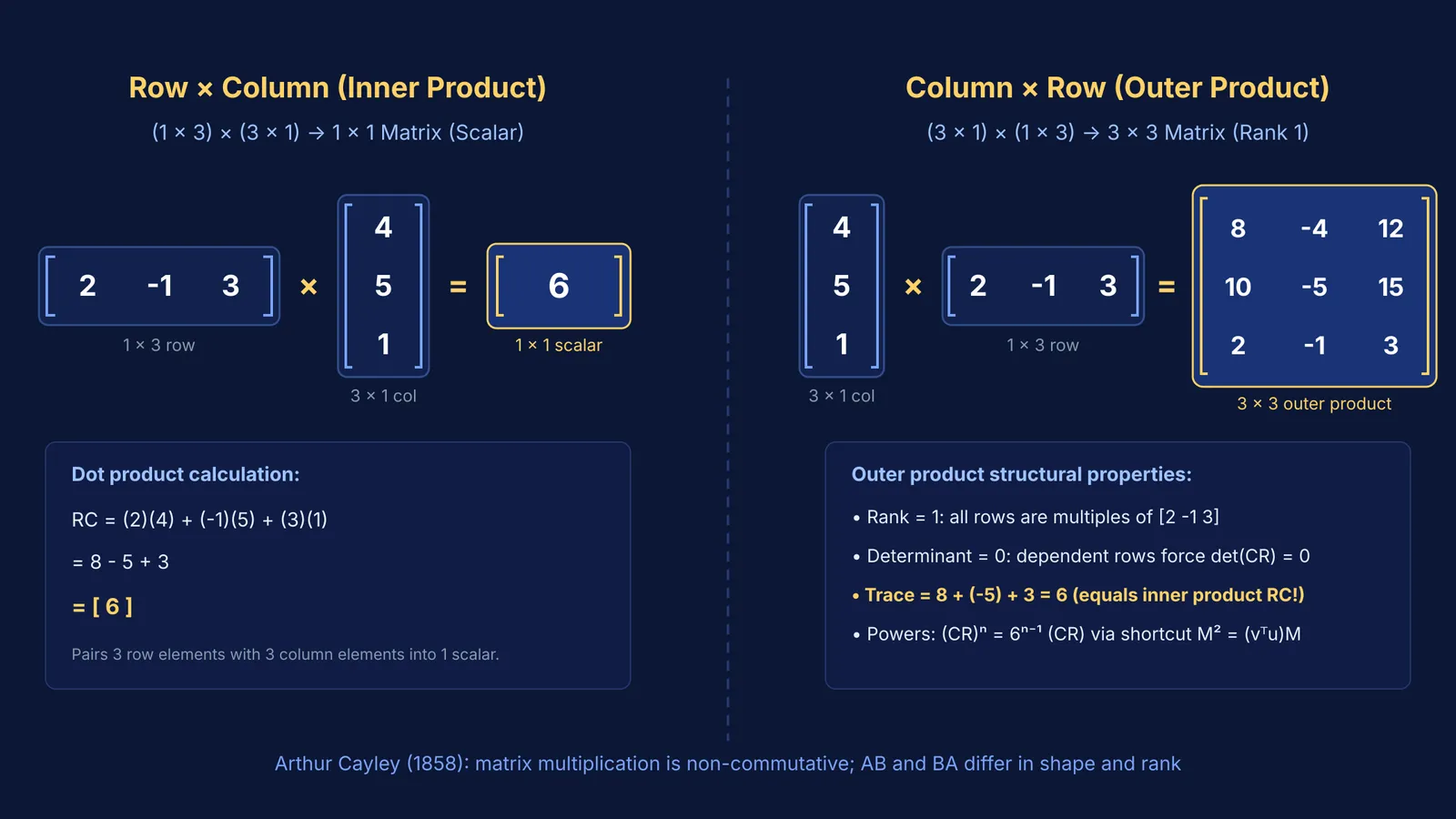
To see the structural contrast between inner and outer products, consider a concrete numerical example with n = 3. Let row matrix R = [2 -1 3] of order 1 × 3, and column matrix C = [4; 5; 1] of order 3 × 1.
The inner product RC multiplies 1 × 3 by 3 × 1:
RC = [(2)(4) + (-1)(5) + (3)(1)] = [8 - 5 + 3] = [6]. The result is a 1 × 1 matrix containing the scalar 6.
The outer product CR multiplies 3 × 1 by 1 × 3:
Row 1: 4 × [2 -1 3] = [8 -4 12]
Row 2: 5 × [2 -1 3] = [10 -5 15]
Row 3: 1 × [2 -1 3] = [2 -1 3]
Assembling these rows creates a 3 × 3 matrix: [8 -4 12] [10 -5 15] [2 -1 3]
Despite containing 9 separate entries, this 3 × 3 outer product possesses three special structural properties:
Rank is exactly 1: Notice that Row 2 is 5/4 times Row 1, and Row 3 is 1/4 times Row 1. All rows are scalar multiples of the original row vector R. Because only one row is linearly independent, the rank of the matrix is 1.
Determinant is zero: Because two or more rows in any n × n outer product (for n ≥ 2) are proportional, its determinant is always 0.
Trace equals the inner product: Adding the main diagonal entries gives 8 + (-5) + 3 = 6. The trace of the outer product CR precisely equals the scalar value of the inner product RC.
How do outer products appear in JEE exam problems?
In competitive entrance examinations administered by the National Testing Agency, examiners frequently test outer products to reward students who recognise algebraic shortcuts over brute-force calculation. A classic problem asks students to compute a high power, such as M¹⁰⁰, for a matrix structured as an outer product M = uvᵀ.
Multiplying M by itself yields:
M² = (uvᵀ)(uvᵀ) = u(vᵀu)vᵀ.
Because vᵀu is a 1 × 1 scalar k, it factors out:
M² = k(uvᵀ) = kM.
By mathematical induction, higher powers satisfy Mⁿ = kⁿ⁻¹ M. For the numerical example above where k = 6, computing CR raised to the power 100 requires no iterative multiplication:
(CR)¹⁰⁰ = 6⁹⁹ (CR).
Recognising this pattern saves valuable minutes during timed tests. You can review similar strategies in our guides on finding powers of a matrix by spotting patterns and matrices and determinants shortcuts for JEE, as well as Arthur Cayley's formulation of matrix algebra.
When tackling challenging multi-step matrix questions, the Fermi Problem Library provides worked problems with a step-by-step solver that explains the reasoning rather than printing an answer. If you find yourself uncertain about whether a product produces a scalar or a grid, Fermi's AI tutor notices where a student is stuck and decides whether to explain, ask or show, helping you master dimensional reasoning from first principles.


