

On this page
When studying chemical kinetics, we often begin with reactions that go to completion. A single reactant A turns into product B with a forward rate constant, k_f. But many reactions are reversible: as soon as B forms, it starts turning back into A with a backward rate constant, k_b.
This opposing process fundamentally changes the math. Instead of dropping to zero, the reactant concentration levels off at an equilibrium state. Understanding how k_f and k_b work together is essential for predicting both where a reversible first-order reaction will end up and how fast it will get there.
What is the rate law for a reversible reaction?
For a simple elementary reversible reaction A ⇌ B, the net rate at which A is consumed depends on two competing terms. The forward reaction uses up A, while the reverse reaction produces more of it.
According to the general rate equation, the net rate of change for the reactant is: d[A]/dt = −k_f[A] + k_b[B]
If we start with an initial concentration of [A]₀ and no product ([B]₀ = 0), then at any time t, the concentration of the product is simply [B] = [A]₀ − [A].
Substituting this into our rate law gives: d[A]/dt = −k_f[A] + k_b([A]₀ − [A])
How do kf and kb set the equilibrium?
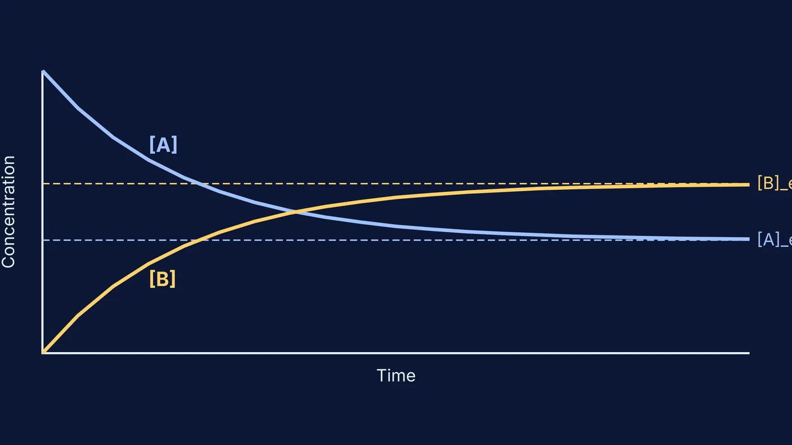
As the reaction proceeds, the forward rate drops (because [A] is falling) and the backward rate rises (because [B] is building up). Eventually, these two rates become equal, and the system reaches dynamic equilibrium.
At equilibrium, the concentrations no longer change, so the net rate d[A]/dt is exactly zero. Setting the forward and reverse rates equal gives: k_f[A]_eq = k_b[B]_eq
Rearranging this reveals that the equilibrium constant K_eq is simply the ratio of the two chemical kinetics rate constants: K_eq = [B]_eq / [A]_eq = k_f / k_b
This tells us where the reaction ends. If k_f is much larger than k_b, the equilibrium lies far to the right, favouring the product. If k_b is larger, the reaction barely seems to happen before settling into a reactant-heavy equilibrium.
Why does the approach to equilibrium depend on (kf + kb)?
The most surprising fact about reversible first-order kinetics is found by solving the differential equation. Integrating the rate law from t = 0 to time t yields: ln( ([A]₀ − [A]_eq) / ([A]_t − [A]_eq) ) = (k_f + k_b)t
Just like with standard integrated rate law graphs, plotting this logarithmic term against time gives a straight line. However, the slope of this line is not just k_f — it is the sum (k_f + k_b).
This means the system approaches equilibrium faster than the forward rate alone would predict. The effective rate constant, often called the observed rate constant k_obs, is k_f + k_b. The reverse reaction acts as a restoring force, pushing the system back towards the middle and shortening the time needed to settle down.
In relaxation kinetics, this rapid return to equilibrium after a small disturbance (like a sudden temperature jump) is measured by a characteristic relaxation time τ. For a first-order reversible reaction, this is defined as τ = 1 / (k_f + k_b) (Wikipedia).
Worked example: Finding the individual constants
In a lab, you cannot easily measure k_f and k_b separately. You can only measure the combined rate of approach to equilibrium and the final equilibrium position.
Suppose a reversible first-order reaction has an observed relaxation rate k_obs = 1.0 × 10⁻³ s⁻¹. When left for a long time, the mixture settles at a ratio of 4:1 in favour of the product, meaning K_eq = 4.0.
To find the individual rate constants, set up a system of two equations:
k_f + k_b = 1.0 × 10⁻³ s⁻¹
k_f / k_b = 4.0
From the second equation, k_f = 4.0 k_b. Substitute this into the first equation: 4.0 k_b + k_b = 1.0 × 10⁻³ s⁻¹ 5.0 k_b = 1.0 × 10⁻³ s⁻¹ k_b = 2.0 × 10⁻⁴ s⁻¹
Then use this to find the forward rate: k_f = 4.0 × (2.0 × 10⁻⁴) = 8.0 × 10⁻⁴ s⁻¹
By observing the single sum and the final ratio, we have extracted the exact speed of both hidden pathways. (Keep in mind that if the temperature changes, both constants will shift, though not always by the exact same temperature coefficient of rate).
If you have concept gaps on how these equations interact, the Fermi Concept Library has every concept in chemistry, each with its own lesson and its place in the map.


