

On this page
In classical mechanics, constant acceleration is the rule for free-falling objects and simple projectiles. But when an object moves through a fluid, such as a microscopic particle settling in water or a boat coasting to a stop, the resistive drag force is proportional to its speed. According to OpenStax University Physics, this low-velocity drag produces a retardation, or negative acceleration, often written as a = −kv.
Because the acceleration keeps changing as the object slows down, the standard constant-acceleration kinematic equations (like v² − u² = 2as or v = u + at) no longer work. Instead, we must use calculus to find how fast the body is going at any moment, and how far it travels before coming to a rest. The maths reveals a fascinating paradox: the body travels a finite distance, but theoretically takes an infinite amount of time to get there.
How to find the distance for a body decelerating with a equals minus k v?
The most direct way to find the stopping distance is to link acceleration to position instead of time. In calculus, we use the chain rule to rewrite acceleration (dv/dt) in terms of distance (x). Since velocity is dx/dt, we can write:
a = dv/dt = (dx/dt) × (dv/dx) = v(dv/dx)
Setting this equal to our given retardation, −kv, we get:
v(dv/dx) = −kv
We can divide both sides by v (assuming the body is still moving and velocity is not zero):
dv/dx = −k
This simple differential equation tells us that the velocity decreases linearly with distance. Integrating both sides with respect to x gives:
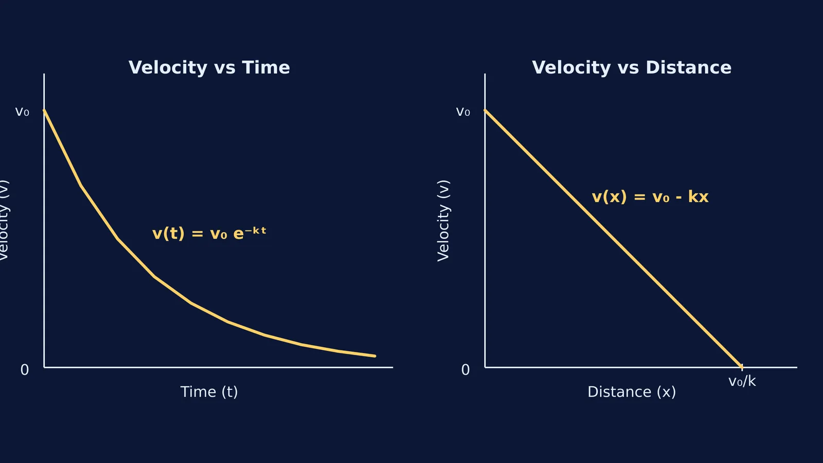
v(x) = v₀ − kx
Here, v₀ is the initial velocity when x = 0. The body stops when its velocity reaches zero. Setting v = 0, we can easily find the total stopping distance:
0 = v₀ − kx
x = v₀ / k
Even though the retardation weakens as the body slows down, it only manages to cover a finite distance. The stopping distance depends entirely on the initial velocity and the drag constant k.
How does velocity change with time?
To find out when the body stops, we return to the time definition of acceleration:
dv/dt = −kv
By separating the variables (grouping v with dv and t with dt) and integrating, we get:
∫ (1/v) dv = −k ∫ dt
Evaluating these integrals from the starting conditions (v = v₀ at t = 0) yields:
ln(v) − ln(v₀) = −kt
Using the properties of logarithms, this becomes:
v(t) = v₀ e⁻ᵏᵗ
This exponential decay means the velocity halves over and over at regular time intervals. Because it keeps halving, it theoretically never reaches zero in a finite amount of time. It approaches a stop asymptotically while its position approaches the maximum distance v₀ / k. In the real world, microscopic random forces eventually take over, but mathematically, the stopping time is infinite.
Where does this happen in physics?
This proportional model appears frequently in problems dealing with linear drag, also known as Stokes' law. As OpenStax notes, for small particles (like bacteria, dust, or silt) moving at low speeds, the viscous drag force is F = 6πηrv. By Newton's second law (F = ma), dividing this resistive force by the particle's mass gives a deceleration proportional to its velocity. It is also used to model boats coasting in water after their engines are turned off.
Variable acceleration requires a solid grasp of calculus, which is easy to set up incorrectly if you pick the wrong substitution. The Fermi Problem Library has worked problems with a step-by-step solver that explains the reasoning rather than printing an answer, helping you choose between using dv/dt or the v(dv/dx) chain rule.
For more on setting up these exact integrals, see how to integrate acceleration given as a function of v or x. If you want to explore the maths of the exponential decay curve, you can review exponential models via dy/dt = ky for similar growth and decay patterns in other subjects.


