

On this page
Reaction kinetics studies how fast products form. The rate law expresses this speed mathematically. But graphing the rate (r) against the concentration of a reactant ([A]) gives a visual fingerprint of the reaction's order.
How does rate vary with concentration on a plot for each order?
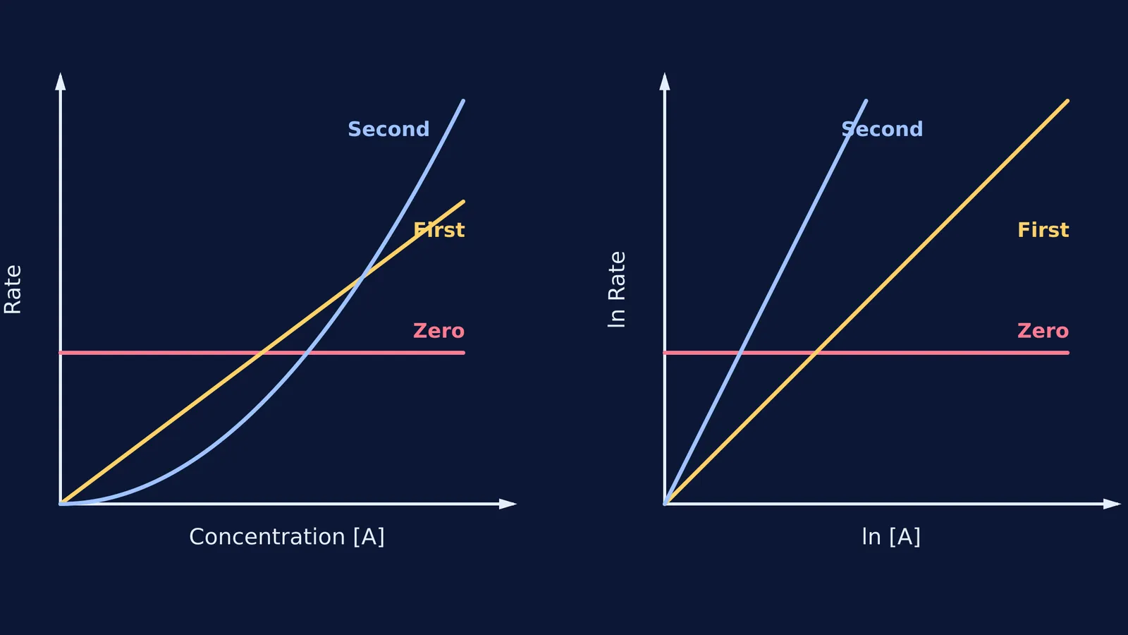
According to Wikipedia's summary of the rate equation, the differential rate law for a single reactant is r = k[A]ⁿ, where k is the rate constant and n is the reaction order. Plotting rate on the y-axis and concentration on the x-axis produces distinct shapes for each integer order:
Zero order (n = 0): The rate is simply r = k. The graph is a flat horizontal line. No matter how much reactant you add, the reaction chugs along at the same constant speed.
First order (n = 1): The rate is r = k[A]. This is the equation of a straight line (y = mx) passing through the origin. The slope of this line is the rate constant k. If you double the concentration, you double the rate.
Second order (n = 2): The rate is r = k[A]². This plots as a parabola curving upwards. As concentration increases, the rate accelerates sharply; doubling the concentration quadruples the rate.
These shapes hold true as long as you isolate one reactant, keeping all other concentrations constant.
When you are wrestling with kinetics problems, a static graph in a textbook can be hard to follow. The Fermi Simulation Lab provides interactive simulations for the ideas that are easier to see than to read. You can adjust concentrations and rate constants on the fly, watching how the curves shift in real time. Because Fermi's AI tutor checks understanding as it goes, it can pause to ask why a second-order parabola climbs so steeply, helping you see the math behind the curve.
Why does a second-order reaction draw a parabola?
A second-order reaction depends on the square of the concentration. In a collision model, this often means two molecules of the same reactant must find each other and collide to react. As the container gets crowded, the number of possible collisions goes up with the square of the number of molecules. This quadratic relationship naturally forms a parabola when graphed.
For a broader look at how reaction rates change with time rather than just concentration, read our guide to Integrated rate law graphs: reading reaction order from straight lines.
How do you find the order from a log-log plot?
Plotting rate against concentration works well for simple integers, but what if the order is fractional, like 1.5? The parabolic curve of 1.5 looks a lot like 2.0 to the naked eye. To find the exact order, chemists use the method of initial rates and a log-log plot. As shown in the rate equation, taking the natural logarithm of both sides of the rate law (ln r = ln k + n ln[A]) turns the power relationship into a linear one.
When you plot the natural logarithm of the rate (ln r) on the y-axis and the natural logarithm of the concentration (ln[A]) on the x-axis:
You get a straight line for any reaction order.
The slope of this line is exactly the partial order (n) of the reaction.
The y-intercept is the logarithm of the rate constant (ln k).
This means a zero-order reaction has a slope of 0, a first-order has a slope of 1, and a second-order has a slope of 2.
If you are stuck calculating these slopes from experimental data, the Fermi Problem Library has worked problems with a step-by-step solver that explains the reasoning rather than printing an answer. Fermi's AI tutor works through problems alongside the student, handling logarithmic conversions step by step. If you need a refresher on logarithms before tackling these slopes, explore the Concept Library, where every concept in mathematics has its own lesson and its place in the map.
What happens to the rate constant in these graphs?
The rate constant k dictates the vertical scale of these plots.
On a standard rate vs concentration plot, a larger k makes the zero-order line sit higher, makes the first-order line steeper, and makes the second-order parabola narrower and taller.
On a log-log plot, changing k shifts the straight line up or down without changing its slope.
According to Wikipedia's article on the Q10 temperature coefficient), a 10 °C change typically doubles the reaction rate, which shifts these graphs upward. For a deeper look, see our post on the Temperature coefficient of rate: why rates double every 10 °C.
A plan for graphing kinetics data
If you are given a table of initial rates and concentrations in an exam or lab, follow this sequence:
Sketch the direct plot: Plot rate against concentration. If it is flat, it is zero order. If it is a straight line through the origin, it is first order.
Convert to logs: If it curves, calculate ln(rate) and ln([A]) for each data point.
Find the slope: Plot the log values. Pick two widely spaced points and calculate the slope (Δy / Δx). That number is your reaction order.
Find k: Read the y-intercept of your log-log line. Calculate e to the power of the intercept to find the rate constant.
By shifting from curves to straight lines, the log-log plot turns a guessing game into a straightforward geometry problem.


