

On this page
When you are asked to find the range of a function on a closed interval, the first step is to check how the function behaves between the endpoints. A continuous function that constantly rises is straightforward, but if the function has turning points, you will need to use calculus to track its highest and lowest values.
Here is how to use the first derivative to determine the range safely, and the steps to follow when the function changes direction.
How do you find the range using monotonicity?
Monotonicity describes whether a function is consistently increasing or decreasing. If the first derivative of a function is positive for all x in an interval, then the function is strictly increasing (Source/04%3A_Applications_of_Derivatives/4.04%3A_The_Mean_Value_Theorem)). This means the curve never dips or flattens out.
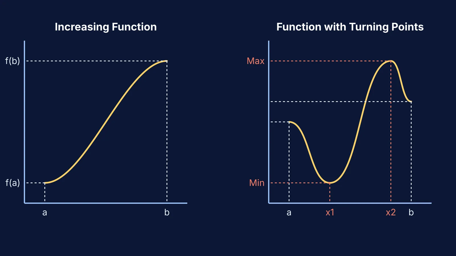
Because an increasing function on a closed interval [a, b] always moves upwards, its lowest point is exactly where it begins, and its highest point is exactly where it ends.
If the function f(x) is continuous and monotonically increasing on [a, b], you do not need to hunt for hidden peaks. You simply calculate the values at the boundaries:
The absolute minimum is f(a).
The absolute maximum is f(b).
The range is the closed interval [f(a), f(b)].
Conversely, if the function is strictly decreasing (its first derivative is always negative), it starts at its highest value and ends at its lowest, making the range [f(b), f(a)].
What if the function has turning points?
If the first derivative changes sign, the function has turning points and is no longer monotonic. You can no longer rely on the endpoints alone to give you the range.
According to the Extreme Value Theorem, if a function is continuous over a closed interval, it must have both an absolute maximum and an absolute minimum (Source/04%3A_Applications_of_Derivatives/4.03%3A_Maxima_and_Minima)). To find the complete range, you have to split the interval at every turning point.
Here is the standard framework for non-monotone functions:
Find the critical points: Find the first derivative f'(x) and set it to zero. Solve for x to find the points where the curve turns flat. Keep only the critical points that fall inside your interval (a, b).
Check the boundaries: Evaluate the original function f(x) at the endpoints a and b.
Check the turns: Evaluate f(x) at every valid critical point.
Compare: The smallest result is your absolute minimum, and the largest result is your absolute maximum. The range is the interval between them.
This method guarantees you will not miss a deep valley or a high peak that occurs in the middle of the interval, a common theme in Absolute maximum and minimum on a closed interval.
A worked example: Range of a non-monotone function
Let us find the range of the function f(x) = x³ − 3x² on the closed interval [−1, 4].
First, we find the derivative to check for monotonicity: f'(x) = 3x² − 6x
Next, we set the derivative to zero to find the critical points: 3x² − 6x = 0 3x(x − 2) = 0
This gives us two critical points: x = 0 and x = 2. Because both 0 and 2 are inside our interval [−1, 4], we must evaluate the function at four places in total (the two endpoints and the two critical points):
At the start (x = −1): f(−1) = (−1)³ − 3(−1)² = −4
At the first turn (x = 0): f(0) = 0³ − 3(0)² = 0
At the second turn (x = 2): f(2) = 2³ − 3(2)² = −4
At the end (x = 4): f(4) = 4³ − 3(4)² = 16
Now, we compare the results. The smallest value is −4, which occurs twice. The largest value is 16. Therefore, the absolute minimum is −4 and the absolute maximum is 16.
The range of the function on this interval is [−4, 16]. You can apply similar logic to rational expressions, as seen in Range of a rational function using the discriminant method.
Where do students go wrong?
The most frequent mistake students make in calculus exams is plugging the endpoints into the function and assuming they have found the range. This shortcut only works if you have already proved the function is strictly increasing or decreasing. If the function has a hidden turning point, skipping the derivative check will give you the wrong answer.
If you find yourself guessing whether a function has turning points, the Fermi Problem Library has worked problems with a step-by-step solver that explains the reasoning rather than printing an answer. It checks your understanding as you go, showing you exactly when and why to take the derivative.
If the rules of calculus feel disconnected, you can review them in the Concept Library, which houses every concept in physics, chemistry, biology, mathematics and computing, each with its own lesson and its place in the map. Taking the time to master these fundamentals ensures you get Domain, range and composite functions done right on exam day.


