

On this page
Why does radial resistance differ from standard wire resistance?
When you first learn Ohm's law in Class 12 physics, resistance is introduced with the familiar formula R = ρL/A. That formula works reliably for an ordinary cylindrical wire because electric current flows longitudinally along its length, passing through a constant cross-sectional area A = πr² over a straight path of length L.
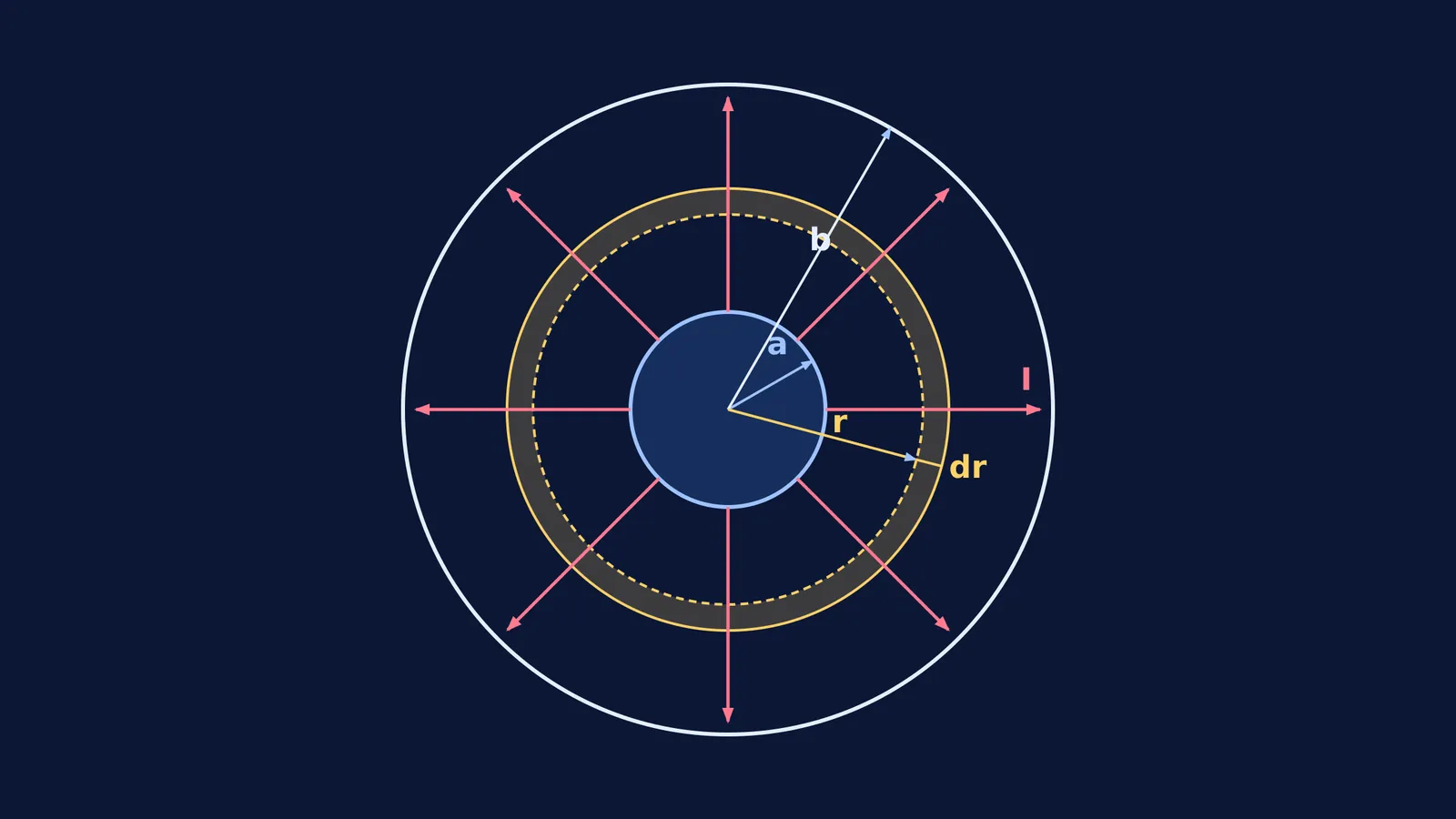
The geometry flips completely when current travels between the inner and outer curved surfaces of a hollow cylinder or coaxial cable. In this configuration, the two electrodes are concentric cylindrical boundaries of length L: an inner surface at radius a and an outer surface at radius b. Current enters at the inner boundary and spreads radially outward in all directions toward the outer boundary. As the current moves outward, the surface area through which it passes is not constant; it expands continuously as 2πrL at every radial distance r. Because the cross-sectional area grows while the path length is directed along the radius dr, you cannot multiply resistivity by a single length-to-area ratio. Instead, you must slice the cylinder into infinitesimal concentric shells in series and integrate their differential resistances.
How do you integrate cylindrical shells to find radial resistance?
To calculate the total radial resistance, consider a thin cylindrical shell of radius r, radial thickness dr, and length L located between the inner radius a and outer radius b.
For this differential shell, electric current flows perpendicular to the cylinder's curved face. The distance the charge carriers travel across the shell is the infinitesimal thickness dr. The cross-sectional area perpendicular to this radial flow is the lateral surface area of the cylinder at radius r, given by A(r) = 2πrL. Using the definition of resistance, the differential resistance dR of this thin shell is:
dR = ρ dr / (2πrL)
Because current must pass consecutively through each concentric shell from radius a to radius b, these differential shells are connected in series. As explained in the textbook OpenStax University Physics Volume 2, the total resistance R between the inner and outer surfaces is obtained by summing these series elements through integration:
R = ∫[a to b] dR = ∫[a to b] (ρ / (2πrL)) dr
Because resistivity ρ, length L, and 2π are constant with respect to radius r, factor them out of the integral:
R = (ρ / (2πL)) ∫[a to b] (1 / r) dr
Evaluating the integral gives the natural logarithm:
R = (ρ / (2πL)) [ln(r)][a to b] = (ρ / (2πL)) (ln b - ln a)
Applying standard logarithm identities yields the final expression:
R = (ρ / (2πL)) ln(b/a)
This result demonstrates two features. First, the resistance depends only on the ratio of the outer to inner radius (b/a), not their absolute difference. Second, the cylinder length L appears in the denominator. A longer cylinder provides a larger lateral surface area for charge leakage, lowering the total radial resistance.
How does radial resistance connect to cylindrical capacitance?
The logarithmic term ln(b/a) in radial resistance is identical to the geometric term that appears in electrostatics. In our guide to spherical and cylindrical capacitors, the capacitance per unit length of two coaxial cylindrical conductors is derived using Gauss's law as C = 2πεL / ln(b/a), where ε is the permittivity of the insulating medium.
When you multiply the radial resistance R of the medium by its capacitance C, the geometric dimensions cancel completely:
RC = [(ρ / (2πL)) ln(b/a)] × [(2πεL) / ln(b/a)] = ρε = ε / σ
Here, σ = 1/ρ is the electrical conductivity of the material. This product, known as the dielectric relaxation time τ = ε/σ, depends exclusively on the intrinsic physical properties of the dielectric material rather than the size or shape of the cylinder. If you know the capacitance of any two-conductor electrode geometry, you can immediately determine the leakage resistance through the surrounding medium without re-evaluating the integral.
The Fermi Concept Library maps every concept in physics, chemistry, biology, mathematics and computing, each with its own lesson and its place in the map, helping students connect electrostatic fields to steady-state current distributions.
Worked example: What is the leakage resistance of a coaxial cable?
In telecommunications and high-voltage transmission, the dielectric jacket between the inner conductor and outer shield experiences a continuous radial leakage current. To see how the formula works with real engineering parameters, consider a standard telecommunication line.
According to ITU-T Recommendation G.621, standard 0.7/2.9 mm coaxial pairs feature an inner copper wire of diameter 0.7 mm (inner radius a = 0.35 mm) and an outer coaxial shield with an inner diameter of 2.9 mm (outer radius b = 1.45 mm). When tested with a DC voltage between 100 V and 500 V, the specification mandates a minimum insulation resistance of 10,000 MΩ·km.
Let us verify the radial resistance for a 1000 m (1 km) section of this cable insulated with high-grade polyethylene possessing a volume resistivity ρ = 4.43 × 10¹⁴ Ω·m:
Radius ratio: b/a = 1.45 mm / 0.35 mm = 4.143.
Natural logarithm: ln(4.143) = 1.4214.
Denominator factor: 2πL = 2 × π × 1000 m ≈ 6283.19 m.
Total radial resistance: R = (4.43 × 10¹⁴ Ω·m / 6283.19 m) × 1.4214 ≈ 1.002 × 10¹¹ Ω.
A resistance of 1.002 × 10¹¹ Ω equals approximately 100,200 MΩ for that 1 km run, satisfying the 10,000 MΩ·km threshold required by ITU-T Recommendation G.621. Notice why cable manufacturers quote insulation resistance in MΩ·km: because radial resistance is inversely proportional to length, multiplying measured resistance by cable length yields a constant benchmark for the dielectric material.
At high alternating frequencies from 1 to 2000 MHz, dielectric conductance and conductor skin depth introduce additional losses, as analyzed by J. S. Bobowski in the American Journal of Physics.
What mistakes do students make in radial integration problems?
In competitive examinations like JEE Advanced, questions on non-uniform current flow frequently test whether you can recognize the direction of current before selecting an integration strategy:
Confusing radial flow with axial flow: When current flows along the axis of a hollow cylinder, the cross-sectional area is the annular ring A = π(b² - a²) and the path length is L, giving R = ρL / (π(b² - a²)). Applying that annular formula to radial current is the single most common mistake on exam papers. Similar setup errors occur when calculating the resistance of a tapered conductor where the radius varies longitudinally instead of radially.
Inverting the length dependence: For axial current, resistance increases proportionally with length, as seen when analyzing how resistance changes with length in a stretched wire. For radial current, doubling the cylinder length doubles the available conduction surface area, halving the overall resistance.
Slicing along the wrong coordinate: You must always choose differential elements whose surfaces are equipotentials. For radial current, every point at radius r shares the same potential, making concentric cylindrical shells the only valid choice.
When solving unfamiliar geometries, the Fermi Problem Library offers worked problems with a step-by-step solver that explains the reasoning rather than printing an answer, ensuring you set up the right differential element on the first attempt.


