

On this page
When you transition from discrete point charges to continuous charged bodies, you can no longer simply plug the total charge into V = kQ/r. Because the charge is spread out, different parts of the body are at different distances from the point where you want to measure the potential.
For a one-dimensional body like a charged rod, the method is to break the rod into tiny, point-like segments and integrate their individual potentials. We will use this continuous charge integration method to find the potential on the axis of the rod.
How do you set up the potential integral?
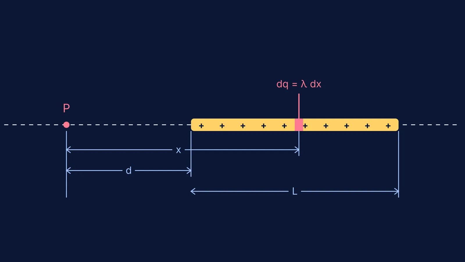
Consider a non-conducting rod of length L with a uniform linear charge density λ = Q/L. We want to find the electric potential V at a point P lying on the axis of the rod, at a distance d from its nearer end.
According to the continuous charge integration principles in OpenStax *University Physics* (source), the total potential at P is the integral of the infinitesimal potentials dV from each charge element dq.
To set this up mathematically, place point P at the origin (x = 0) and align the rod along the positive x-axis so that it spans from x = d to x = d + L.
Take an infinitesimally small slice of the rod of length dx at a position x. The charge of this slice is dq = λ dx.
The distance from this slice to the origin is exactly x. Therefore, the small contribution to the potential at P from this slice is dV = kλ dx / x.
How do you integrate kλ dx / x?
To find the total potential, we integrate this expression from the start of the rod to the end:
V = ∫ kλ (dx / x)
Because k and λ are constants, they pull out of the integral, leaving us to integrate 1/x from x = d to x = d + L. The integral of 1/x is the natural logarithm, ln(x). Evaluating this at the upper and lower limits gives:
V = kλ [ln(x)] from d to d + L = kλ (ln(d + L) − ln(d))
Using the logarithm rule ln(a) − ln(b) = ln(a/b), the final formula is:
V = kλ ln((d + L) / d)
If we replace λ with Q/L, we can also write this as:
V = (kQ / L) ln(1 + L/d)
This exact expression underscores why physics requires calculus: the potential scales logarithmically with distance rather than following the simple 1/r rule of a point charge. Setting up the integral is often where students stumble. If you are practising these derivations for JEE, the Fermi Problem Library has a step-by-step solver that explains the reasoning for choosing your coordinate system and integration limits.
What happens to the potential far away?
In physics, checking extreme cases is a powerful way to verify a formula. What happens if we move point P very far away, so that d is much larger than L?
When L/d is very small, we can use the mathematical approximation ln(1 + x) ≈ x for small values of x.
Applying this to our formula yields V ≈ (kQ / L) × (L / d) = kQ / d.
From far away, the rod's length becomes negligible, and its electric potential looks exactly like that of a point charge of magnitude Q.
How do you calculate the potential step by step?
Identify the given values: d = 2.0 m, L = 4.0 m, Q = 6.0 × 10⁻⁶ C, and k = 9.0 × 10⁹ N m²/C².
Calculate the linear charge density: λ = Q / L = (6.0 × 10⁻⁶ C) / 4.0 m = 1.5 × 10⁻⁶ C/m.
Apply the formula: V = kλ ln((d + L) / d).
Substitute the numbers: V = (9.0 × 10⁹) × (1.5 × 10⁻⁶) × ln((2.0 + 4.0) / 2.0).
Simplify the expression: V = 13500 × ln(3).
Since ln(3) is approximately 1.0986, V ≈ 14831 V.
The potential is approximately 1.48 × 10⁴ V.
If you want to master continuous charge distributions, similar methods apply to calculating the potential at the centre of a uniformly charged solid sphere. You can also use this result to verify the rod's electric field using the rule for an electric field from a potential gradient.


