

On this page
In short Graphing a piecewise function requires evaluating the boundary points for each rule, using an open circle for strict inequalities like < and a closed circle for inclusive ones like ≤. Education research (DOI: 10.29333/iejme/255) shows that focusing on the whole function as a unified process helps prevent the common mistake of treating each piece as a completely separate graph.
Many students are comfortable graphing standard curves like y = x² or straight lines like y = 3 − x. But when a single function uses different rules for different intervals of x, it breaks the expectation of a smooth, single-equation curve.
Researchers note that this clash often causes errors. A 2010 study in the *International Electronic Journal of Mathematics Education* found that action-oriented teaching—which focuses purely on procedural rules—confines students to an "action conception," making them treat the pieces as entirely separate functions rather than one unified mathematical object (DOI: 10.29333/iejme/255).
To sketch these functions accurately and pass the vertical line test, you have to read the domain intervals carefully, mark your breakpoints, and know exactly where each piece stops.
How do you mark the breakpoints?
A piecewise function is split by boundary values in its domain. For example, consider:
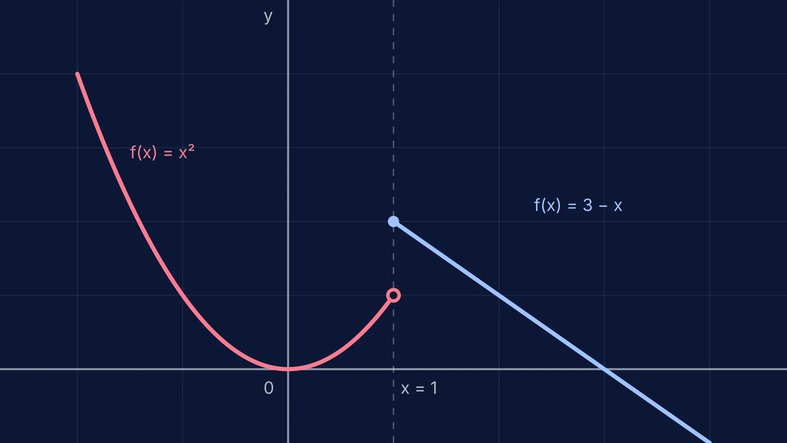
f(x) = x² if x < 1 f(x) = 3 − x if x ≥ 1
The breakpoint here is x = 1. A reliable way to start your graph is to draw a faint, vertical dashed line at this boundary. This line acts as a visual wall: the parabola y = x² is strictly forbidden from crossing to the right of x = 1, and the line y = 3 − x cannot cross to the left.
Because many functions defined this way deal with absolute values, you can see similar split-domain logic when solving equations and inequalities with modulus.
When do you use open and closed circles?
At the breakpoint, the two pieces of the graph might meet, or they might have a vertical "jump". To show exactly what happens at the boundary x-value, you must plug the breakpoint into the equations and mark the coordinates with the correct type of circle, as standard educational materials emphasize (Khan Academy).
Open Circle (○): Used for strict inequalities (< or >), meaning the point is not included in the domain of that piece.
Closed Circle (●): Used for inclusive inequalities (≤ or ≥), meaning the point is part of the graph.
In our example, at the boundary x = 1, the first piece is y = x² for x < 1. Plugging in 1 gives y = 1. Because the inequality is strictly less than (<), you draw an open circle at (1, 1).
For the second piece, y = 3 − x for x ≥ 1. Plugging in 1 gives y = 2. Because this inequality includes "equal to" (≥), you draw a closed, solid circle at (1, 2).
If you are struggling to picture why the rules change at these specific boundaries, the Fermi Concept Library covers every concept in mathematics, each with its own lesson and its place in the map.
A step-by-step framework for graphing
To prevent overlapping lines and domain errors, use this sequence for every piecewise function:
Draw boundary walls: Lightly sketch vertical dashed lines at every x-value where the function's rule changes.
Evaluate the limits: Plug the boundary x-values into the corresponding pieces to find their endpoints, even for strict inequalities.
Place the dots: Draw open or closed circles at those endpoints based on the inequality symbols.
Plot the intervals: Pick one or two test x-values inside each restricted domain (e.g., x = -1 and x = 0 for the x < 1 piece). Plot those points and connect them to the boundary circle.
Erase the excess: Make sure no line extends past its designated boundary wall.
Reading domain and range from the result
Once the graph is drawn, you can verify its overall domain (the valid x-inputs) and range (the resulting y-outputs).
Look at the diagram at the top of this page. The domain spans all real numbers, because the open circle at x = 1 is covered by the closed circle above it. The range (the vertical span of the graph) also spans all real numbers. As you move left, the parabola climbs towards positive infinity. As you move right, the line piece starts exactly at y = 2 and goes downwards to negative infinity. Together, they cover every possible y-value, so the range is (−∞, ∞).
Checking these bounds graphically is similar to evaluating limits at infinity of rational functions—you are looking at how the function behaves at its extreme ends and boundaries. If you find evaluating these boundary conditions confusing, the Fermi Problem Library has a step-by-step solver that explains the algebraic reasoning rather than just printing an answer.


