

On this page
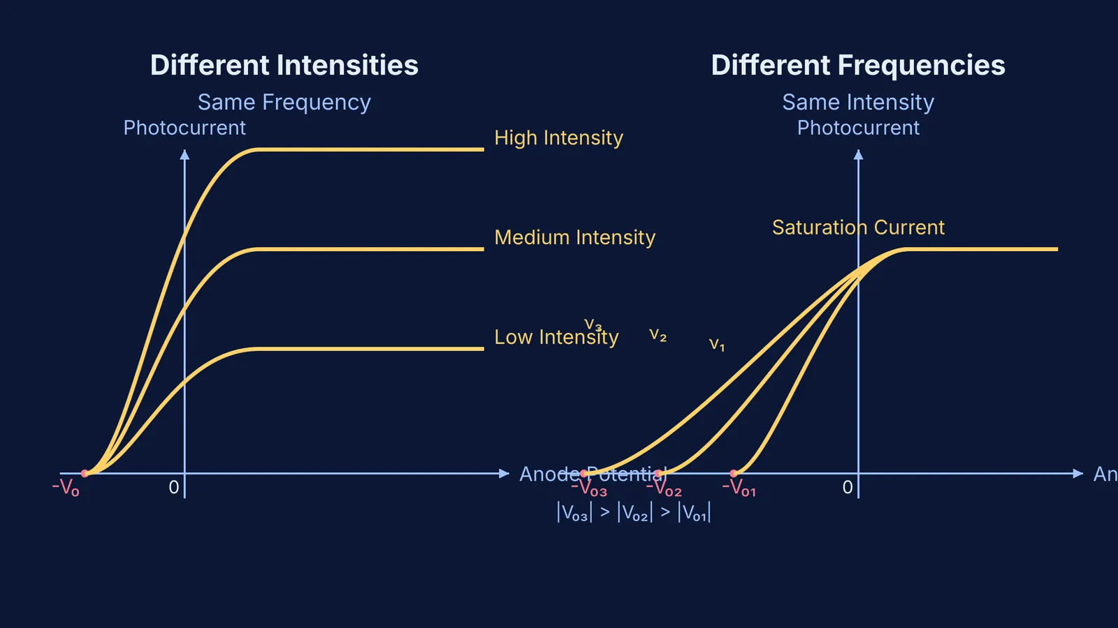
When you study the photoelectric effect for exams like JEE and NEET, two graphs appear in almost every past paper: the variation of photocurrent with anode potential.
One graph shows what happens when you change the intensity of the incident light. The other shows what happens when you change its frequency. They test whether you understand the fundamental difference between the *number* of photons and the *energy* of each photon.
Here is how to read both curves without getting them mixed up.
What is the photocurrent vs anode potential graph?
In a photoelectric tube, light strikes a metal plate (the cathode) and knocks out electrons. These electrons travel to the collector plate (the anode), creating a photocurrent.
When you apply a positive potential to the anode, it pulls the electrons in. Eventually, all emitted electrons are collected, and the current reaches a maximum value called the saturation current.
When you apply a negative (retarding) potential to the anode, it repels the electrons. Only the fastest electrons make it across. At a specific negative voltage, even the most energetic electrons are turned back, and the current drops to zero. This is the stopping potential (−V₀), and it measures the maximum kinetic energy of the emitted electrons. You can find a detailed breakdown of these terms in the OpenStax University Physics text.
If you are solving problems based on photon counts, you can read more about finding the number of photons emitted per second by a lamp or a laser.
How does the photocurrent vs anode potential graph change for different intensities?
When you increase the intensity of the light while keeping its frequency constant, the graph grows taller but starts at the exact same point on the horizontal axis.
Saturation current increases: Higher intensity means more photons are striking the metal per unit of time. Since one photon ejects one electron, a higher photon flux means more photoelectrons, which creates a larger saturation current.
Stopping potential remains constant: The energy of each individual photon (E = hν) has not changed. Therefore, the maximum kinetic energy of the ejected electrons remains exactly the same, so the identical retarding voltage is needed to stop them.
If you see a graph with multiple curves branching up to different heights but all originating from a single −V₀ on the left, it shows varying intensities (I₃ > I₂ > I₁).
How does the photocurrent vs anode potential graph change for different frequencies?
When you increase the frequency of the light, the graph stretches further to the left, but all curves flatten out at the same height.
Stopping potential becomes more negative: Higher frequency means each photon packs more energy. By Einstein's photoelectric equation (K_max = hν − Φ), the ejected electrons have greater kinetic energy. You need a stronger negative voltage to stop them, so the stopping potential shifts further to the left (|V₀₃| > |V₀₂| > |V₀₁|).
Saturation current remains constant: In the standard textbook model, "constant intensity" in this context implies a constant number of incident photons per second. Since the same number of electrons are ejected per second, the saturation current does not change.
*(Note: To quickly calculate the energy of these photons in electron-volts, you can use the E = 1240/λ formula).*
How do you solve exam questions on these graphs?
When you encounter these graphs in an exam, check the axes and the starting points immediately:
Look at the left (x-axis intersection): If the curves start at different points, the frequency is changing. The curve starting furthest to the left has the highest frequency.
Look at the right (flat plateaus): If the curves flatten out at different heights, the intensity is changing. The highest curve has the highest intensity.
Check the material: If both the stopping potential and the saturation current change simultaneously in a way that doesn't fit the rules above, the question might be comparing two entirely different photosensitive metals with different work functions.
To master these curve-shifting concepts, you need to practice them in varying contexts. You can explore worked examples with a step-by-step solver in the Fermi Problem Library.


