On this page
When you first learn about electrical current, you often treat it as flowing evenly through a wire. If the current density J is constant, the total current is just the density multiplied by the cross-sectional area: I = J × πR².
However, many advanced physics problems ask what happens when the current density varies with the radial distance from the centre of the wire, r. This non-uniform distribution requires setting up an integral over the cross-section. We see this principle in action in high-frequency alternating current, where current crowds toward the outside edge of a wire, or in specialised semiconductor designs where doping profiles change across the material.
How do you find total current with current density varying with radius?
To find the total current I, you must integrate the current density J(r) over the cross-sectional area. The general rule is I = ∫ J · dA (OpenStax University Physics Volume 2).
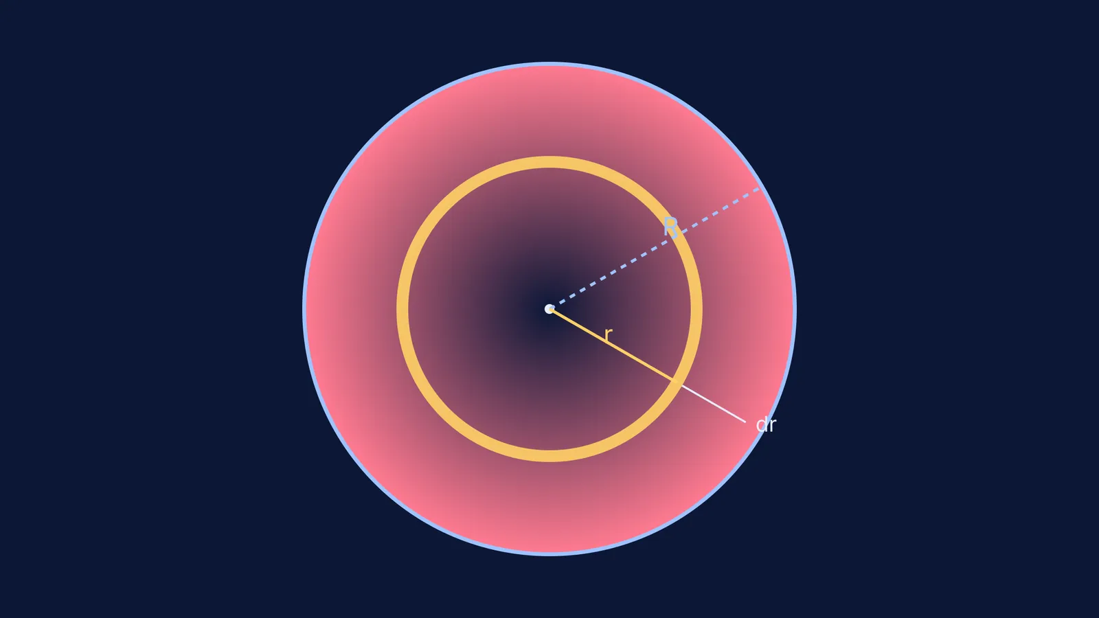
For a cylindrical wire, the current flows perpendicularly through the circular cross-section. Because the density changes only with the radius r, we slice the area into thin concentric rings. A ring at radius r with a tiny thickness dr has an area:
dA = 2πr dr
The current flowing through this single thin ring is dI = J(r) × 2πr dr. To find the total current in a wire of radius R, you sum up all these rings by integrating from the centre to the edge (from 0 to R):
I = ∫ J(r) 2πr dr
If struggling to set up integrals is holding you back in problems like Resistance of a tapered conductor: setting up the integral, the Fermi Concept Library builds from the basic geometry of these slices up to the calculus.
What is the formula for current density varying linearly with radius?
A common exam problem states that the current density increases linearly from the axis of the wire to its surface. This is written as J(r) = kr, where k is a constant.
To solve this, substitute J(r) = kr into the integral:
I = ∫ (kr) 2πr dr
Pull the constants 2πk out of the integral:
I = 2πk ∫ r² dr
Integrate r² to get r³/3, and evaluate it from 0 to R:
I = 2πk [R³/3 − 0]
I = 2πkR³ / 3
This result is much smaller than if you had simply multiplied the maximum surface density by the total area. If you misapply the uniform area formula to non-uniform fields, the Fermi Problem Library will point out the mistake and show you the exact reasoning required.
How do you calculate the average current density?
Once you have the total current, you might be asked to find the average current density across the whole wire.
The average current density is simply the total current divided by the total cross-sectional area:
Average J = I / (πR²)
Using our previous linear example where I = 2πkR³ / 3, the average density is:
Average J = (2πkR³ / 3) / (πR²) = 2kR / 3
This tells you that the average density is exactly two-thirds of the maximum density (kR) found at the wire's surface.
How do you solve a worked example with a varying current density?
Let us put numbers to the formula. Suppose a cylindrical wire of radius R = 2 mm (which is 0.002 m) has a current density that varies with the radius according to J(r) = (5 × 10⁶ A/m³) r. What is the total current flowing through the wire?
First, identify the constant k = 5 × 10⁶ A/m³.
Substitute the values into the formula we derived above:
I = 2πkR³ / 3
I = 2π × (5 × 10⁶ A/m³) × (0.002 m)³ / 3
Calculate the radius cubed:
(0.002)³ = 8 × 10⁻⁹ m³
Now multiply the terms:
I = 2π × (5 × 10⁶) × (8 × 10⁻⁹) / 3
I = 2π × (40 × 10⁻³) / 3
I ≈ 0.251 / 3 ≈ 0.0838 A
The total current flowing through the wire is 83.8 mA.
How do you handle other non-uniform profiles?
You will use this exact same framework for any radial profile. For example:
Quadratic variation (J = Cr²): The integral becomes 2πC ∫ r³ dr, which evaluates to πCR⁴ / 2.
Decreasing density (J = J₀(1 − r/R)): You split the integral into two parts: 2πJ₀ ∫ r dr minus (2πJ₀/R) ∫ r² dr.
The logic matches what you do when finding the charge enclosed in Gauss's law for a sphere with non-uniform charge density or calculating the Energy density in an electric field across a volume. You identify the thin geometry where the physical value is constant, set up the area or volume element, and integrate from the centre to the boundary.