

On this page
When data is grouped into class intervals, you can no longer see the exact raw numbers to find the most frequent value. Instead, you have to find the "modal class"—the group that contains the highest concentration of data—and then mathematically estimate where the mode lies within that group.
For students preparing for board exams or competitive tests like JEE, applying the mode formula for grouped data is a standard skill. Yet, it is easy to make calculation errors or misidentify the components of the formula. In this article, we explain how to locate the modal class, how the formula interpolates the result, and the most common pitfalls you need to avoid.
What is the modal class?
The modal class is defined as the class interval that has the highest frequency in a given data set [[1]](https://en.wikipedia.org/wiki/Mode_(statistics)).
When looking at a frequency distribution table, your first step is to scan the frequency column for the largest number. The interval that corresponds to that maximum frequency is your modal class. The actual mode of the entire data set is guaranteed to fall somewhere inside this range.
A common mistake is writing down the maximum frequency itself as the answer. For example, if the 20–30 interval has a frequency of 15, and 15 is the highest frequency in the table, the modal class is "20–30", not "15". The frequency just points you to the correct interval.
How do you apply the mode formula?
Since we do not know the exact individual values inside the modal class, we must estimate. We assume the mode is positioned inside the modal class based on the "pull" of the frequencies in the neighbouring classes [[1]](https://en.wikipedia.org/wiki/Mode_(statistics)). If the class before it has a higher frequency than the class after it, the mode shifts toward the lower end of the interval [[1]](https://en.wikipedia.org/wiki/Mode_(statistics)).
We calculate this exact position using the mode formula:
Mode = L + (f₁ - f₀) / (2f₁ - f₀ - f₂) × h
Here is how to extract each term from your table:
L: The lower limit of the modal class.
h: The size (or width) of the class interval. You find this by subtracting the lower limit from the upper limit of the modal class.
f₁: The frequency of the modal class itself.
f₀: The frequency of the class immediately preceding (before) the modal class.
f₂: The frequency of the class immediately succeeding (after) the modal class.
Why does the mode formula use this geometric interpolation?
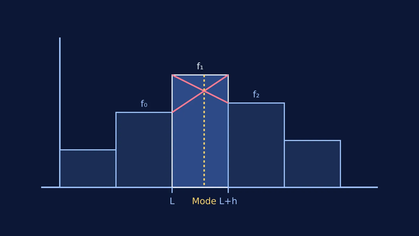
When you look at a histogram of grouped data, the tallest bar represents the modal class. However, the true peak of the distribution is rarely exactly in the middle of that bar.
The mode formula calculates the peak by creating a geometric intersection. Imagine drawing a diagonal line from the top-left corner of the modal class bar to the top-left corner of the bar immediately after it. Then, draw another line from the top-right corner of the modal class bar to the top-right corner of the bar immediately before it.
The point where these two diagonal lines cross is the estimated mode. If the bar before the modal class is taller than the bar after it, the intersection gets pulled toward the left side of the modal class. If the bar after it is taller, the intersection shifts to the right. The mathematical formula we use is simply a way to calculate the exact coordinate of that crossing point without having to draw the graph. This visual method ensures we account for the influence of the immediately surrounding data points.
What if the modal class is the first or last group?
Students frequently drop marks because they use the wrong values for the adjacent frequencies, especially when the modal class sits at the very edge of the data table.
The modal class is the first group: If the very first interval has the highest frequency, there is no "preceding class" in the table. In this case, you simply set f₀ to 0.
The modal class is the last group: Similarly, if the modal class is at the bottom of the table, there is no succeeding class. Here, f₂ becomes 0.
Handling these boundary cases properly ensures your calculation does not break down at the extremes of your data.
How do you handle discontinuous intervals?
Another common error happens when the class intervals are not continuous. If your classes look like 10–19, 20–29, and 30–39, you cannot just use L = 20 and h = 9 for the modal class.
The mode formula requires continuous boundaries. You must first close the gaps by subtracting 0.5 from the lower limits and adding 0.5 to the upper limits. Your intervals become 9.5–19.5, 19.5–29.5, and 29.5–39.5. Now, for the middle class, L becomes 19.5 and the true class size h is 10. Always check your table for continuity before you start extracting your variables.
If you find yourself stuck on statistics problems or repeatedly making boundary errors when calculating central tendencies, the Fermi Problem Library has worked problems with a step-by-step solver that explains the reasoning behind each formula substitution rather than just printing an answer.


