

On this page
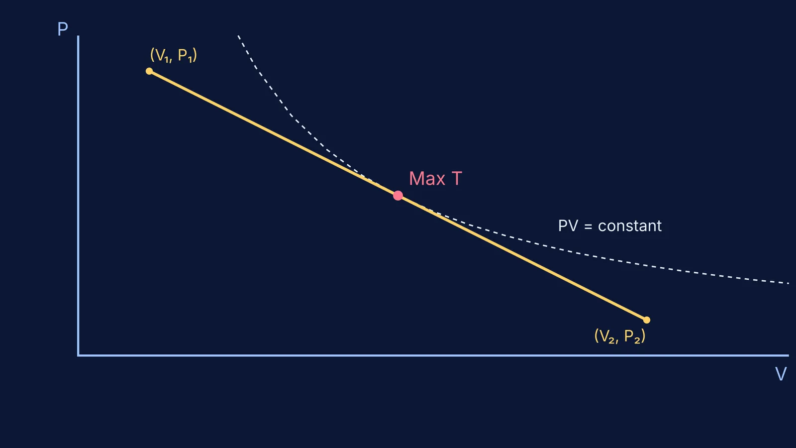
When students first encounter thermodynamics, they usually learn a few standard paths: isothermal (constant temperature), isobaric (constant pressure), and adiabatic (no heat exchanged). But what happens when an ideal gas expands along an arbitrary straight line on a pressure-volume (PV) diagram?
The temperature does not stay constant. It rises to a peak and then falls back down. Finding that peak is a classic exam problem that tests whether you can connect a graphical representation to the ideal gas equation.
Why do arbitrary lines confuse us?
It is tempting to look at a straight line on a graph and assume it belongs to a familiar category. Students often attempt to force every straight-line process into the rules of isothermal or adiabatic changes. A seminal 2004 study found that only 20% or fewer of university physics students can make effective use of the first law of thermodynamics even after instruction.
When pressure (P) drops linearly as volume (V) increases, the process is neither isothermal nor adiabatic. Because PV = nRT, the temperature (T) depends on the product of pressure and volume. As the gas expands along the line, the increasing volume initially outpaces the dropping pressure, driving the temperature up. Eventually, the shrinking pressure wins, and the temperature falls again.
How do you write temperature as a function of volume?
To find the exact maximum, we write temperature entirely in terms of volume.
The equation of a straight line with a negative slope on a PV diagram is: P = −mV + c where m is the positive magnitude of the slope and c is the y-intercept.
From the ideal gas law, we know: T = PV / nR
Substitute the linear equation for P into the temperature equation: T = (−mV + c)V / nR T = (−mV² + cV) / nR
This shows that temperature is a quadratic function of volume. Because the V² term is negative, the graph of T against V is a downward-opening parabola, confirming that the temperature reaches a single maximum peak.
Where does the maximum temperature occur?
To find where this maximum occurs, we differentiate T with respect to V and set the derivative to zero: dT/dV = (−2mV + c) / nR = 0
Solving for V gives the volume at the maximum temperature: V_max = c / 2m
We can plug this volume back into our linear equation to find the corresponding pressure: P_max = −m(c / 2m) + c = c / 2
Notice what these coordinates mean. If you extend the straight line segment all the way to the axes, it intersects the volume axis at V = c/m and the pressure axis at P = c. The point (c/2m, c/2) is exactly halfway between those two intercepts.
Once you can handle a single linear segment, the next step is tackling a full cyclic process loop area to find the net work. You might also need to practice converting PV, PT and VT graphs to see how the same process looks from different angles.
Is heat flow zero at the maximum temperature?
A common misconception is that the point of maximum temperature must be the point where the gas stops absorbing heat and starts releasing it.
This is incorrect. The point of maximum temperature is where the linear process is perfectly tangent to an isotherm (a curve of constant temperature). However, heat flow reverses when the process becomes tangent to an adiabat (a curve where no heat is exchanged). Because adiabatic curves are steeper than isothermal curves, the gas actually continues to absorb heat for a short time even after its temperature has begun to drop. During this brief window, the gas exhibits a negative molar heat capacity.
If you are struggling to set up the calculus or visualize the curves, the Fermi Concept Library can help. Fermi's AI tutor works out what you already know and builds a plan for the session—drawing the figure and checking understanding as it goes, so you sit down to a clear next step.


