

On this page
In short
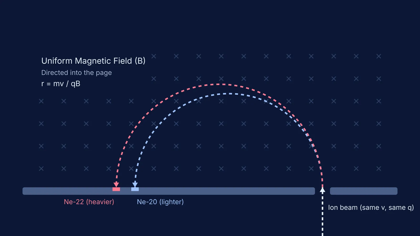
In a mass spectrometer, a magnetic field separates isotopes because heavier ions are harder to deflect, causing them to travel in a wider arc. When ions of the same charge and speed enter the field, their path's radius depends entirely on their mass, a property used to discover the first stable isotopes in 1912.
How does a magnetic field separate isotopes?
When atoms are ionised (given a positive charge by removing electrons) and accelerated, you get a beam of charged particles. If you pass this beam through a velocity selector, only ions travelling at one exact speed emerge. At this point, the beam contains a mix of isotopes—atoms of the same element with the same charge and speed, but different masses.
As the beam enters a uniform magnetic field, the ions experience a magnetic force at right angles to their motion. This perpendicular force acts as a centripetal force, pushing the ions into a circular path. Because the heavier isotopes have more momentum, the magnetic field cannot bend their path as sharply as it bends the path of the lighter ones. They travel in a wider semicircle, landing farther along a detector plate.
Why does the radius depend on mass?
We can prove this by equating the magnetic force to the centripetal force required to keep the ion moving in a circle.
For an ion with charge q and speed v moving perpendicular to a uniform magnetic field B, the magnetic force is F = qvB. The centripetal force needed to maintain a circle of radius r is F = mv²/r.
Setting these equal gives: qvB = mv²/r
Solving for the radius of the path r: r = mv/qB
In a properly calibrated mass spectrometer, the charge q, speed v, and magnetic field B are identical for every ion in the beam. The only variable that changes is the mass m. Therefore, the radius is directly proportional to the mass (r ∝ m). A heavier isotope will have a proportionately larger radius of curvature.
How did the mass spectrometer prove isotopes exist?
Before this principle was put to work, chemists assumed that every atom of a given element was identical. That changed when physicists began passing charged gases through magnetic and electric fields.
In 1912, the British physicist J. J. Thomson used a primitive version of this setup on neon gas and noticed two distinct landing spots on his photographic plate. This was the first evidence that a stable element could have isotopes (Neon-20 and Neon-22). His student Francis William Aston refined the technique, building the first mass spectrograph. Aston's work revealed that many non-radioactive elements are actually mixtures of isotopes, earning him the 1922 Nobel Prize in Chemistry. Today, we use these isotopic signatures for everything from Clair Patterson and how lead isotopes dated the Earth to calculating the Average atomic mass from isotope abundance: worked problems.
Calculating the separation distance: a worked example
Let's look at exactly how far apart Thomson's two neon isotopes would land in a typical textbook problem.
Suppose a beam of singly charged Neon-20 and Neon-22 ions enters a magnetic field of 0.5 T at a constant speed of 1.0 × 10⁵ m/s. Both have a charge of q = 1.6 × 10⁻¹⁹ C. First, we find the mass of each isotope in kilograms. Using 1 u ≈ 1.66 × 10⁻²⁷ kg:
Mass of Neon-20: m₂₀ = 20 × 1.66 × 10⁻²⁷ kg = 3.32 × 10⁻²⁶ kg
Mass of Neon-22: m₂₂ = 22 × 1.66 × 10⁻²⁷ kg = 3.65 × 10⁻²⁶ kg
Next, we use r = mv/qB to find the radius of each path. For Neon-20: r₂₀ = (3.32 × 10⁻²⁶ × 1.0 × 10⁵) / (1.6 × 10⁻¹⁹ × 0.5) = (3.32 × 10⁻²¹) / (0.8 × 10⁻¹⁹) = 4.15 × 10⁻² m So, the radius is 4.15 cm.
For Neon-22: r₂₂ = (3.65 × 10⁻²⁶ × 1.0 × 10⁵) / (0.8 × 10⁻¹⁹) = 4.56 × 10⁻² m So, the radius is 4.56 cm.
The ions complete a semicircle, meaning they strike the detector at a distance of 2r from the entrance slit.
Neon-20 hits at 2 × 4.15 cm = 8.30 cm
Neon-22 hits at 2 × 4.56 cm = 9.12 cm
The separation distance on the plate is 9.12 − 8.30 = 0.82 cm, or 8.2 mm. This distinct gap makes it easy to measure the relative abundance of each isotope.
If you want to visualise how changing the speed or the magnetic field strength alters these trajectories, try mapping them out in the Simulation Lab. For step-by-step practice with the r = mv/qB formula and other electromagnetism topics, you can explore the Concept Library hub.


