

On this page
Every linear programming problem (LPP) is built on limits. You want to maximise profit or minimise cost, but you are constrained by supplies of time, materials or budget. In mathematical modelling, these limits are written as linear inequalities. Plotted on a coordinate plane, they create a feasible region. But what happens when constraints contradict?
When does a linear programming problem have no solution?
A linear programming problem breaks down and yields no solution when its constraints are mutually contradictory.
According to the official textbook for NCERT Class 12 Mathematics (Chapter 12), the feasible region is the common region determined by all constraints, including non-negativity conditions x ≥ 0 and y ≥ 0. If the inequalities point in opposite directions, their intersection is empty. Because no coordinate point (x, y) can satisfy every condition simultaneously, the problem is termed infeasible, and no optimal solution can exist.
Why does an empty feasible region break the model?
To solve an LPP, we rely on the corner point method in linear programming. This theorem states that if an optimal solution (a maximum or minimum) exists, it must occur at one of the corner points, or vertices, of the feasible region.
As documented in Wolfram MathWorld's optimization reference, the feasible region contains all points satisfying every constraint. When constraints clash, this region is empty. Without shared space or boundary vertices, there are no corner points to test in the objective function, making it mathematically impossible to calculate an optimal value.
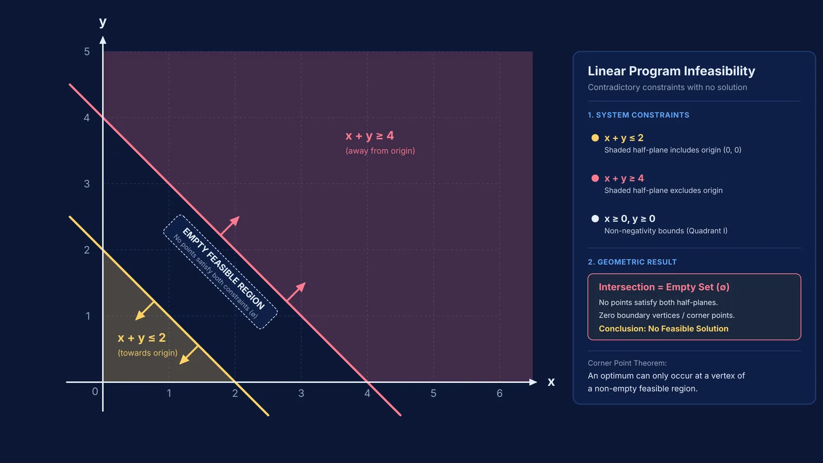
Consider a manufacturing model with conflicting targets. If one constraint mandates using at most 2 units of material (x + y ≤ 2), while another requires producing at least 4 units of output (x + y ≥ 4), the model breaks. No non-negative numbers can sum to less than 2 and simultaneously sum to 4 or more.
How do you spot an empty region on a graph?
When graphing linear inequalities on paper, an empty region is easy to spot through three deliberate checks:
Draw the boundary lines: Convert each inequality into an equation, plotting x + y = 2 and x + y = 4 as straight lines across the first quadrant.
Shade the half-planes: Test the origin (0, 0). For x + y ≤ 2, (0, 0) satisfies the inequality (0 ≤ 2), so shade towards it. For x + y ≥ 4, (0, 0) fails (0 ≥ 4), so shade away from it into the upper quadrant.
Check the intersection: The feasible region is strictly where all shaded areas overlap. If the half-planes point in opposite directions with an unshaded gap between them, the intersection is empty.
How do empty and unbounded regions differ?
Students often confuse empty regions with unbounded regions. While graphing inequalities—whether using linear systems or the wavy curve method for inequalities—the geometric shape determines what solution to expect:
Infeasible (Empty Region): There are zero valid points. The shaded half-planes never overlap, meaning the problem has no solution.
Unbounded Region: The overlap exists but extends infinitely in one or more directions. The problem has infinite feasible points. While a minimum cost might still occur at a lower boundary vertex, a profit objective like Z = 5x + 3y grows infinitely, leaving no finite maximum.
How can you fix an infeasible problem?
If an optimization problem produces an empty feasible region, use this troubleshooting plan to identify and resolve the underlying error:
Check non-negativity: Verify that you have shaded only within the first quadrant, respecting x ≥ 0 and y ≥ 0.
Verify inequality directions: Re-read problem wording carefully. Phrases like "at most" translate to ≤, while "at least" means ≥. Reversing them is a common trap.
Test constraints independently: Plot constraints one by one. If you want to practice setting up inequalities, the Fermi Problem Library offers worked problems with a step-by-step solver that explains the reasoning rather than printing an answer.
Look for redundant or conflicting rules: Real-world models sometimes include too many constraints. Dropping an overly restrictive, non-essential requirement can restore the feasible region and allow optimization.


