

On this page
When students first encounter calculus, "local maximum" intuitively sounds like a high mountain peak, and "local minimum" sounds like a low valley. It is easy to assume that any maximum on a curve must be greater than any minimum. Yet in calculus, a local maximum can be strictly smaller than a local minimum. Understanding why this happens comes down to a single word students often overlook: "local."
Can a local maximum really be less than a local minimum?
Yes. The words "maximum" and "minimum" in calculus describe the geometry of individual turning points, not the overall height of a curve. According to OpenStax Calculus Volume 1, a function f has a local maximum at c if there exists an open interval I containing c such that f(c) ≥ f(x) for all x in I. Conversely, f has a local minimum at c if there exists an open interval I containing c such that f(c) ≤ f(x) for all x in I.
The crucial word is "interval." A local extremum only competes against its immediate neighbours within that open window. When a curve has multiple branches or sharp shifts, a local peak in one region can easily sit lower than a local valley elsewhere.
How does the function x + 1/x prove this mathematically?
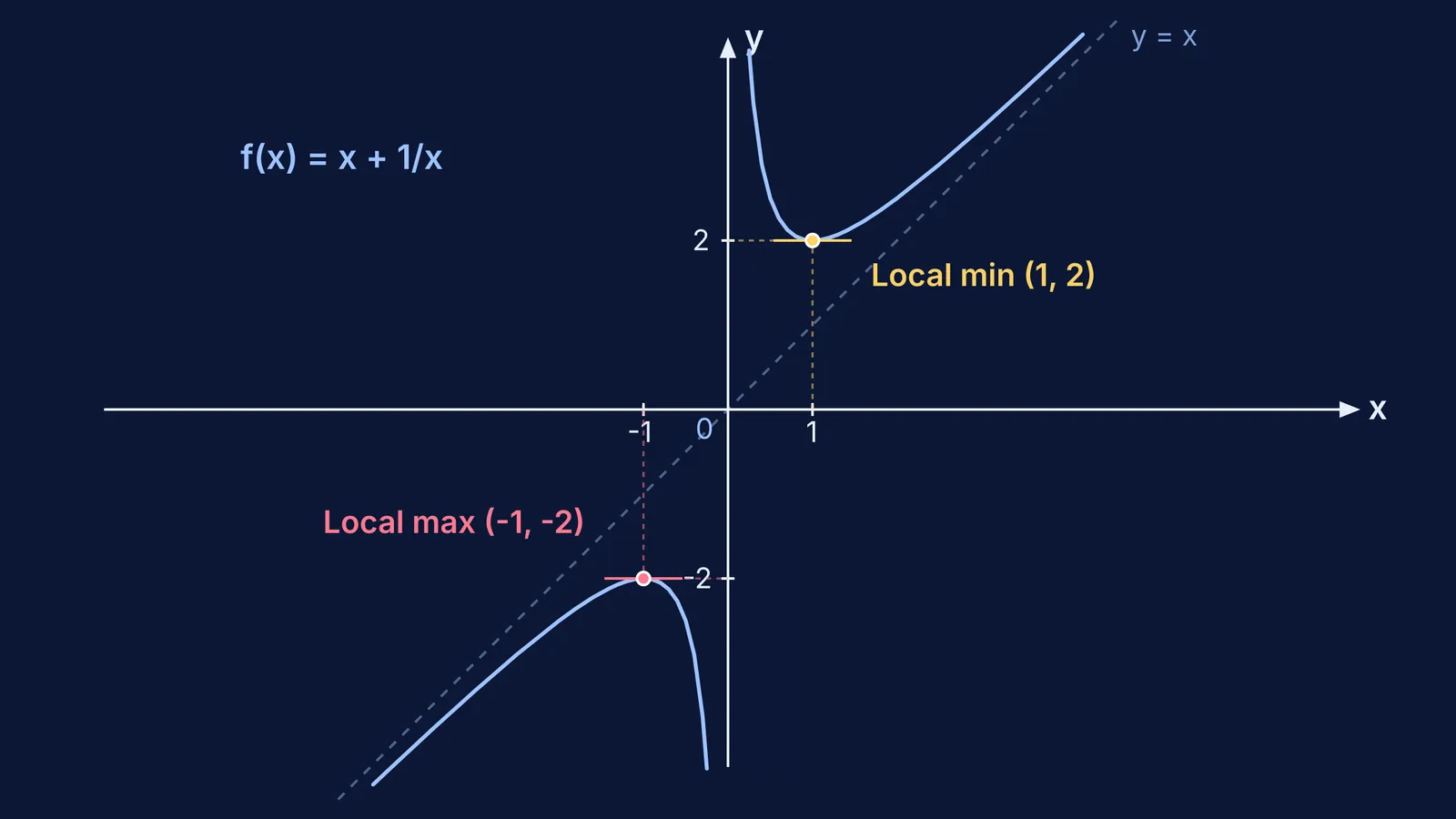
The classic demonstration is the rational function f(x) = x + 1/x, defined for all non-zero real numbers x. Its domain is (−∞, 0) ∪ (0, ∞), separated by a vertical asymptote at x = 0.
To find its stationary points, calculate the first derivative: f′(x) = 1 − 1/x² = (x² − 1) / x². Setting f′(x) = 0 gives x² − 1 = 0, yielding two critical points at x = 1 and x = −1.
Testing concavity with the second derivative, f″(x) = 2/x³, classifies both points:
At x = −1: f″(−1) = 2/(−1)³ = −2 < 0. Because the curve is concave downward, x = −1 is a local maximum, with value f(−1) = −1 + 1/(−1) = −2.
At x = 1: f″(1) = 2/(1)³ = 2 > 0. Because the curve is concave upward, x = 1 is a local minimum, with value f(1) = 1 + 1/1 = 2.
The local maximum value is −2, while the local minimum value is 2. Because −2 < 2, the local maximum is strictly smaller than the local minimum. As mathematician Paul Dawkins notes in Paul's Online Math Notes, relative extrema describe only local peaks and valleys within a small neighbourhood, so a relative maximum does not have to exceed a relative minimum elsewhere.
Why does everyday intuition confuse local and global extrema?
Everyday language treats "maximum" as an absolute superlative—the highest possible amount. In mathematics, that concept is the global (or absolute) maximum, which must indeed be greater than or equal to any global minimum on the same domain.
In the CBSE Class 12 Mathematics curriculum, the unit on Calculus carries 35 marks out of 80, with the second derivative test forming a core method in the Application of Derivatives chapter. Board and JEE Main questions frequently test whether students distinguish local turning points from overall bounds. On bounded domains, you must check endpoints alongside critical points; see our guide on absolute maximum and minimum on a closed interval.
Derivatives also govern where the curve climbs and falls; see our walkthrough of increasing and decreasing functions. Furthermore, f(x) = x + 1/x never takes values strictly between −2 and 2, which you can confirm using the range of a rational function using the discriminant method.
How can you test for local extrema without making graphing errors?
Follow this 4-step checklist to evaluate extrema accurately:
State the domain: Identify non-zero conditions or vertical asymptotes that split the graph into disconnected branches.
Locate all critical points: Differentiate the function and find all values in the domain where f′(x) = 0 or where f′(x) does not exist in the domain.
Classify each point: Use the first or second derivative test to check local concavity and turning direction.
Separate local peaks from global bounds: Check end behavior as x approaches infinity or domain boundaries before claiming an absolute extreme.
When working through multi-step calculus problems for school boards or competitive exams like JEE Main, identifying critical points and setting up sign charts can feel tedious. The Fermi Problem Library offers worked problems with a step-by-step solver that explains the reasoning rather than simply printing a final answer. To build a clear mental model of how turning points, discontinuities, and asymptotes interact across rational curves, you can explore the Fermi Concept Library, where every concept in mathematics has its dedicated lesson and its place in the topic map.


