

On this page
When you solve a linear programming problem (LPP) on a graph, the standard approach is to check the coordinates of every corner of your feasible region to see which gives the highest profit. But there is a faster, more visual way: the isoprofit line method.
By drawing one line that represents a fixed profit and sliding it across your graph, you can instantly see where the objective function reaches its peak. First developed by Soviet mathematician Leonid Kantorovich in 1939 (Wikipedia), linear programming relies on this geometric relationship to find optimal outcomes efficiently.
Why do we use the isoprofit line method?
The usual technique, the corner point method, requires you to find the exact coordinates of every vertex of your feasible region. If your region has many constraints, calculating the intersection points for all of them takes time.
The isoprofit line method skips the arithmetic. Instead of calculating the profit at every corner, you use the slope of the objective function to spot the winning corner visually. Because the slope depends only on the coefficients of your variables (for example, -a/b for an objective function Z = ax + by), every isoprofit line is parallel to the others. This means you only need to plot one line accurately.
How do you slide the isoprofit line?
An isoprofit line represents all the combinations of x and y that give the exact same total profit. Mathematically, it is a level set of the cost function.
Here is how to use it:
Draw the feasible region: Plot your constraint inequalities and shade the region where they overlap. When exploring how different constraints change the feasible region, remember that the Fermi Concept Library has every concept in physics, chemistry, biology, mathematics and computing, each with its own lesson and its place in the map.
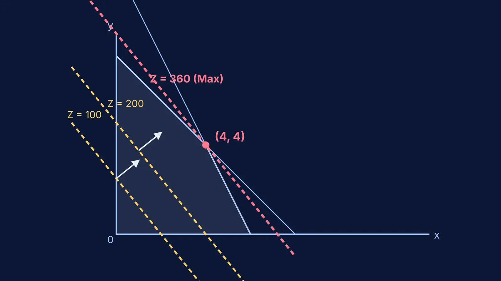
Draw a starting line: Pick a convenient, small value for your objective function (Z = ax + by), and draw that line on your graph. This gives you your baseline slope.
Slide the line: Because all isoprofit lines for a given objective function have the same slope, you can lay a ruler on your starting line and slide it parallel to itself. Move it away from the origin to increase Z. The direction you slide depends on whether the coefficients in your objective function are positive or negative.
Find the last point: The optimum of the linear cost function is where its level set intersects the polygon farthest in the direction of optimization (Wikipedia). The last corner your sliding line touches before leaving the feasible region is your maximum.
If you find setting up these constraints difficult, the Fermi Problem Library has worked problems with a step-by-step solver that explains the reasoning rather than printing an answer.
What is the isocost method for minimizing?
Linear programming is not just about maximizing profit; it is also used to minimize costs (like the amount of material or time used).
When your goal is to minimize the objective function, the technique is exactly the same, but the direction changes. You draw an initial "isocost" line and slide it *toward* the origin. The last point the line touches before it shrinks away from the feasible region entirely is your minimum cost. This method works perfectly as long as your feasible region is bounded near the origin.
For more on visual problem-solving, read our guide on finding roots by curve intersections, or learn how to split cases in modulus equations and inequalities.


