

On this page
Finding the inverse of a matrix usually involves a long, multi-step process. You must find minors, build a matrix of cofactors, transpose it to find the adjoint, and finally divide by the determinant. For a 2×2 matrix, this entire process reduces to a quick, three-step shortcut.
What is the shortcut for the inverse of a 2×2 matrix?
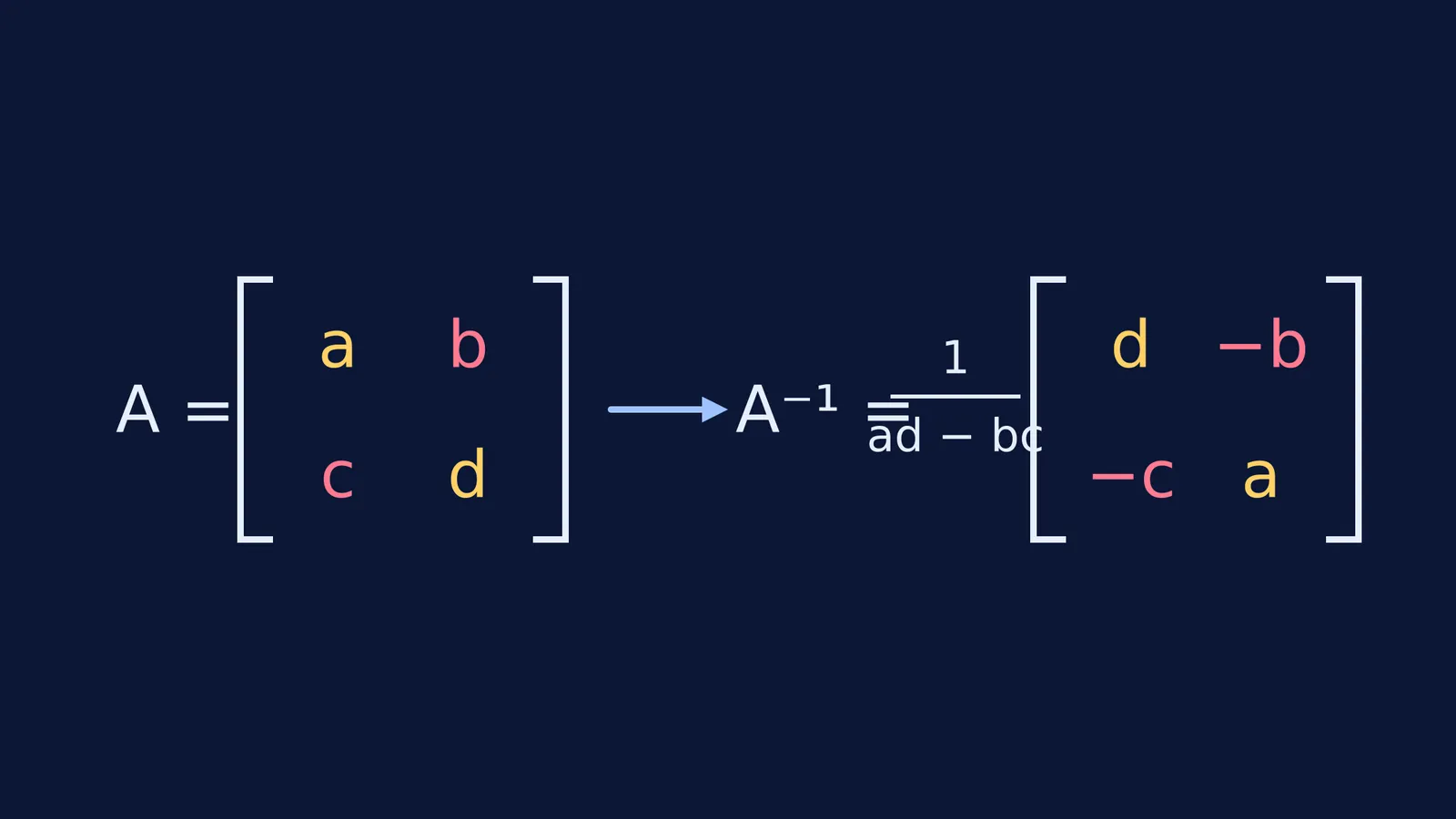
If you have a 2×2 matrix A with elements a, b, c and d arranged in two rows:
A = [ a b ] [ c d ]
Its inverse, A⁻¹, is given directly by the formula:
A⁻¹ = [ 1 / (ad − bc) ] × [ d −b ] [ −c a ]
The inverse of a 2×2 matrix is found by swapping the main diagonal elements, negating the other two elements, and dividing the result by the matrix's determinant (mathcentre). According to a guide from the UK's mathcentre, this works in three specific steps:
Swap the diagonal: Exchange the positions of the elements on the leading diagonal (a and d).
Negate the off-diagonal: Multiply the other two elements by −1 (change b to −b, and c to −c), leaving them in their original positions.
Divide by the determinant: Divide every element in the new matrix by the original matrix's determinant, which is calculated as ad − bc.
A worked example
Let's find the inverse of the matrix M:
M = [ 4 7 ] [ 2 6 ]
First, we apply the swap and negate rules to the matrix elements.
Swap the diagonal: The 4 and 6 change places.
Negate the off-diagonal: The 7 becomes −7, and the 2 becomes −2.
The adjusted matrix is now: [ 6 −7 ] [ −2 4 ]
Next, we divide by the determinant. The determinant of M is the product of the main diagonal minus the product of the off-diagonal: (4 × 6) − (7 × 2) = 24 − 14 = 10.
Multiply the adjusted matrix by 1/10:
M⁻¹ = 1/10 × [ 6 −7 ] [ −2 4 ]
You can leave it with the 1/10 outside as a scalar multiplier, or distribute it inside to get decimal values:
M⁻¹ = [ 0.6 −0.7 ] [ −0.2 0.4 ]
If you make a sign error when negating or swapping, the Fermi Problem Library has a step-by-step solver that explains the reasoning rather than printing an answer, helping you catch the mistake early.
Example 2: Handling negative numbers
The rule applies exactly the same way when the original matrix already contains negative numbers. Let's find the inverse of N:
N = [ −3 5 ] [ −2 4 ]
First, find the determinant: (−3 × 4) − (5 × −2) = −12 − (−10) = −2. Since the determinant is not zero, the inverse exists.
Swap the diagonal: The −3 and 4 change places.
Negate the off-diagonal: The 5 becomes −5, and the −2 is negated to become positive 2.
The adjusted matrix is: [ 4 −5 ] [ 2 −3 ]
Now, divide by the determinant (−2):
N⁻¹ = 1/(−2) × [ 4 −5 ] [ 2 −3 ]
Distributing the −1/2 gives the final inverse:
N⁻¹ = [ −2 2.5 ] [ −1 1.5 ]
This second example highlights why the step is called "negate" rather than "make negative." You are flipping the sign, so an originally negative off-diagonal element becomes positive.
When does a matrix not have an inverse?
The shortcut requires dividing by the determinant, ad − bc. If the determinant evaluates to exactly zero, the formula collapses because you cannot divide by zero.
A square matrix with a determinant of zero is called a singular matrix, and it does not have an inverse (mathcentre). Before applying the swap and negate steps, it is always best practice to calculate the determinant first. If it is zero, you can stop immediately—the matrix is singular.
How to check if your inverse is correct?
The fundamental definition of an inverse is that multiplying a matrix by its inverse must return the identity matrix, I.
A · A⁻¹ = I
For a 2×2 matrix, the identity matrix I is: [ 1 0 ] [ 0 1 ]
To verify that the shortcut worked for our first example, we multiply M by M⁻¹:
[ 4 7 ] · [ 0.6 −0.7 ] [ 2 6 ] [ −0.2 0.4 ]
Using the standard row-by-column matrix multiplication rule:
Top left: (4 × 0.6) + (7 × −0.2) = 2.4 − 1.4 = 1
Top right: (4 × −0.7) + (7 × 0.4) = −2.8 + 2.8 = 0
Bottom left: (2 × 0.6) + (6 × −0.2) = 1.2 − 1.2 = 0
Bottom right: (2 × −0.7) + (6 × 0.4) = −1.4 + 2.4 = 1
The result is exactly the identity matrix. This proves the shortcut successfully found the true inverse. Once you master this rule for 2×2 matrices, you can explore the adjoint and inverse of a matrix for larger grids, or look at how finding Aⁿ for a matrix behaves when multiplied repeatedly.


